.png)
This post continues from the previous post: Towards 2-Dimensional State-Space Models (2): WHippo.
Let’s recap the principles of state-space models (SSMs) we have settled in the previous post.
- The main equation of the SSMs is determined by two components:
compression function and input transformation . - SSM’s goal is to let the network distill the property of the compression function , by mimicking its behavior under the input transformation .
- We can manually derive the compression function’s dynamics , and let the hidden state follow the dynamics to behave as a “compressed” state.
- SSMs often let the compression function be a projection using 1D orthogonal basis functions and define as a token concatenation, leading them to obtain a compression function dynamics in a form of following differential equation:
where is a token that appears at the -th timestep.
- WHippo suggests letting be a 2D orthogonal polynomial projection and be a Gaussian blurring, which ends up yielding:
The most noticeable difference is the existence of the input term . This difference emerges from the fact that we do not define the input transformation as an information-adding manner; in fact, it is rather a information-losing process, since the information of a blurred image is strictly a subset of the information of the sharper image .
In fact, it was my original attempt; we can derive the relationship between two coefficients and using the information gap between two images , which becomes:
Due to the linearity of the basis projection , our resulting equation ends up feeling a bit underwhelming. Note that the whole point of SSM is to get the network to distill the properties of compression function . This formulation guides the network to obtain linearity, which indeed is a property of , but it is not exactly the most unique property of the compression function.
You might be able to derive non-trivial equation if you choose other than basis projections (such as PNG or H.264); but I leave it as a future exploration as of now.
As a result, we no longer can stick to the traditional way of sequence modeling, where the model updates the hidden state depending on the inflowing new tokens.
State-space modeling as a regularization
Thus, the WHippo’s state update needs to happen only in a form of regularization, rather than an explicit update like how 1D SSMs do.
For instance, let us define a parameterized feature extractor and say, we want this feature extractor to produce hidden states: . Then, we can regularize to follow the proposed dynamics Eq. (2)Show information for the linked content by the following loss :
where is a distance measure.
Enabling SSM’s principles in such a way gives a somehow intriguing advantage:
The SSMs enabled with the regularization loss are now independent from the model ’s architecture. Hence, we can adopt the SSM’s principle without explicitly using the well-known SSM blocks such as S4, S4D, or S5. Here I omit Mamba since we are dealing with linear-time invariant (LTI) SSMs at least for now.
However, this is where WHippo becomes harder to be compared with other SSMs, since its performance largely varies by the architecture we choose for .
An interesting usage of the state-space regularization
From now on, I’ll call the regularization loss from Eq. (3)Show information for the linked content the state-space regularization for future reference.
I was wondering where this regularization could become useful and discovered that this can provide a quite niche value in image tokenization.
What is image tokenization?
Well, in the modern era of AI, everything happens in a latent space—onto which the input is projected in order to be handled in a lighter, interpretable way.
Image tokenizer often provides a way to represent RGB images in a form of tokens: they are easier to handle for neural networks compared to RGB image, and often encode image semantics that pixel values cannot provide.
The most common use case of this tokenization is generation, since the tokenization greatly reduces the number of tokens to process, and this can help accelerating the resource-demanding generation process by the order of magnitude.
The research trends in world models or representation learning have also been shaping toward latent modeling these days, so the value of this tokenization is rising continuously. One of my recent publications also features this, so check it out!
Anyway, in this post, let’s focus only on tokenization for generation, as this area is where state-space regularization becomes valuable.
A good image tokenization
What defines a good image tokenization? There could be several but at this point, the following two are the most important factors:
- Reconstruction fidelity: an image tokenizer should recover images sufficiently well from the latent tokens.
- Generation-friendliness: an image tokenizer should provide generation-friendly latent space, where the latent distribution is easily modeled with existing generation models.
Reconstruction fidelity being a good property is quite obvious: the tokens should hold the image information accurately in a fixed token budget in order to properly represent a pixel-heavy image. See thisShow information for the linked content for the reference; the detail of the castle has changed significantly, and that is often not regarded as a good reconstruction.
Generation-friendliness matters if you are planning to use the tokenizer to any type of generation tasks; which may include image generation/editing, planning, or manipulation—and all of them stand in the middle of AI research right now.
The problem is that nobody actually knows what makes a tokenizer "generation-friendly" yet. Right now, the only way to find out is to train a full generative model from scratch and see how it performs. As you can guess, that burns through massive amounts of time and money, and that is exactly why researchers are trying to find a shortcut—a way to measure or improve a tokenizer's generation capability before the generative model training. Below are some notable efforts:
- EQ-VAE, FT-SE: enforcing rotation- or scale-equivariance between latent and pixel spaces helps.
- MAETok: latent space represented with fewer Gaussian modes helps.
- VA-VAE, RAE, ReDi: involving vision foundation model helps.
- UL: directly involving a diffusion prior helps.
A noteworthy theory in this field is that reconstruction fidelity and generation-friendliness are hardly achieved together.
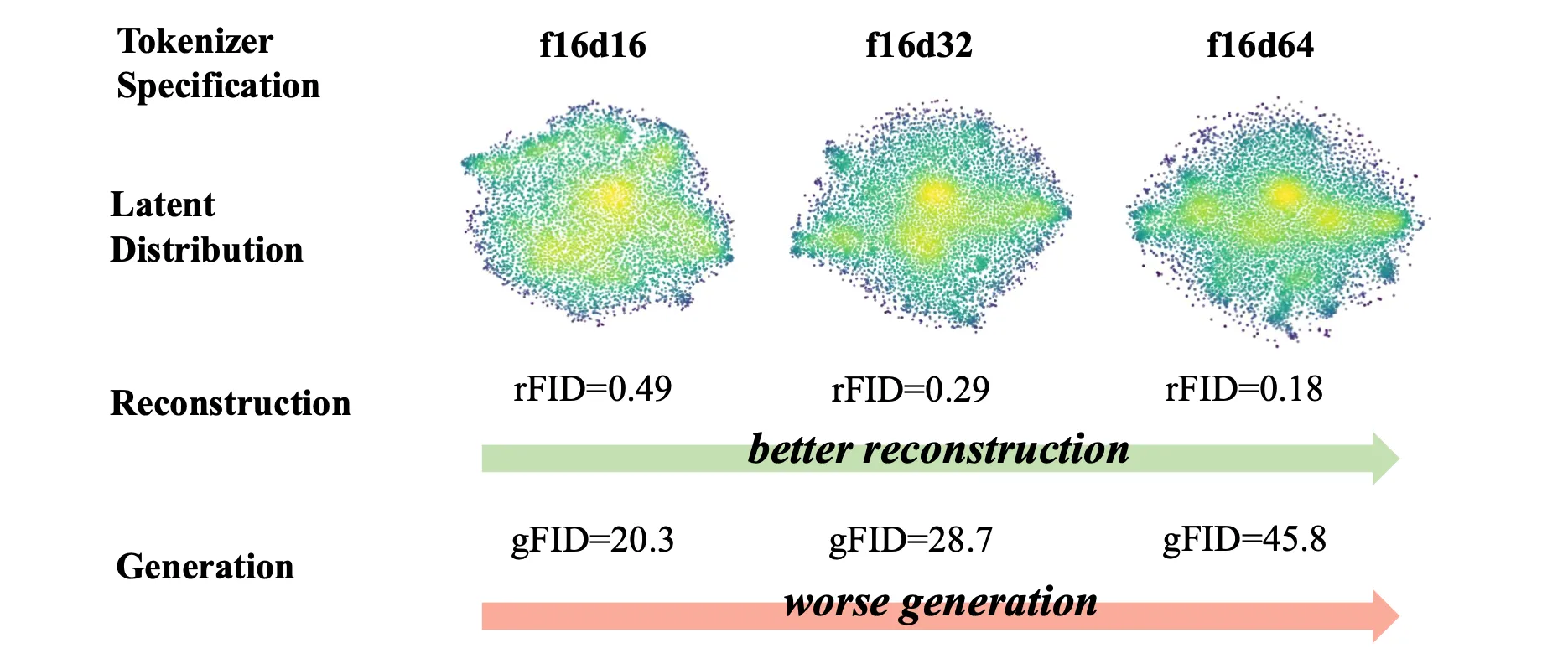
The better a tokenizer reconstructs the input image, the more you will have to give up a certain degree of generation quality. To intuitively explain, pushing a tokenizer to better reconstruct the input often make tokens have to encode pixel-perfect details of an image, thereby creating immense complexities in the latent distribution, making generative models hard to learn the latent distribution.
Why would state-space regularization help?
We thought our state-space regularization might help achieving both at the same time for two reason:
- Our regularization nudges the hidden state (here, the latent feature) to resemble the compression function, so there is a chance of it producing more compact latent features.
- Choosing basis projections as compression function enables the latent to capture spectral components of the input, which helps generative models to synthesize images in a structured order.
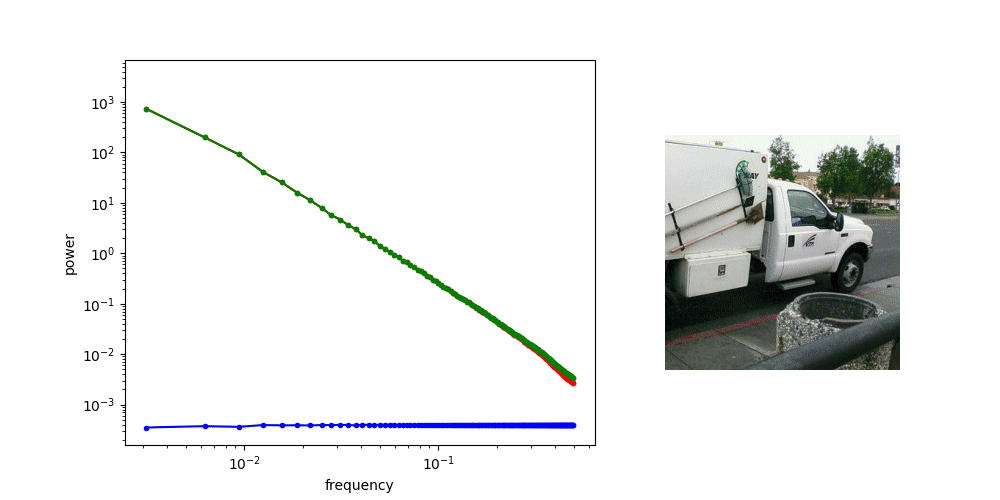
The second claim is primarily based on a famous insight delivered from Generative Model with Inverse Heat Dissipation or Diffusion is Spectral Autoregression: diffusion models generate images by first generating low-frequency components of images, and then the high-frequency details. Recent studies in this field often explicitly design diffusion to happen in such order, achieving better generation quality.
State-space regularization applied to image tokenizers
We designed our regularization to be applied to an image tokenizer as follows:
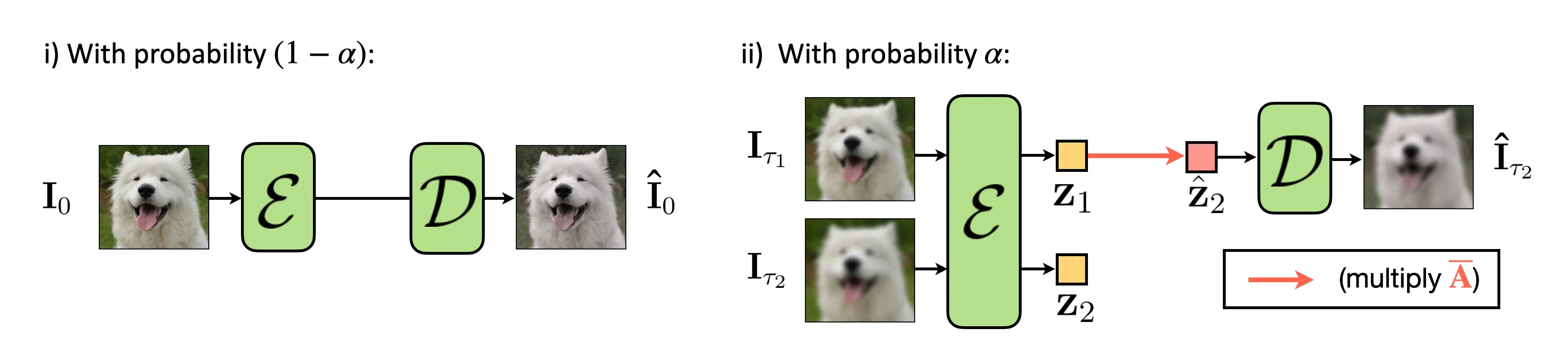
Regularization strength indicates how often a tokenizer should focus more on creating relationships between two latents rather than reconstructing the input. Through this way, we can make latents of a sharper image and a blurrier image follow the predefined basis coefficients dynamics. Hence, we can expect each channel of a latent will behave as if it is a coefficient of 2D orthogonal polynomials.
A few interesting properties emerged from the regularization
We analyzed how the state-space regularization affects the latent, and observed some interesting behaviors that the regularization brings.
- Blurring translates to a simpler dynamics in the latent space.
The following two animations illustrate the latent space where 100 images are projected onto, plotted using 2 PCA basis. The trajectory that each point draws shows how each latent behaves when the corresponding image is blurred.
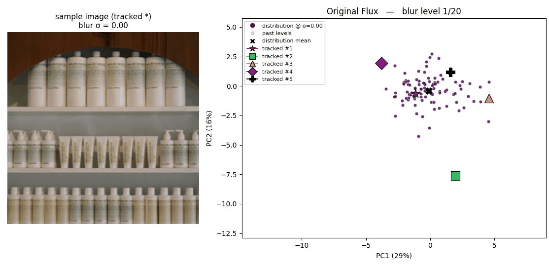
How latents from the original Flux tokenizer behave 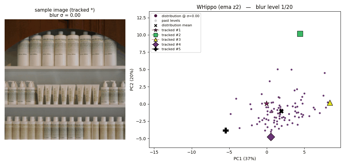
How latents from the regularized tokenizer behave The regularized latent space tends to show simpler dynamics; which is expected regarding that our regularization enforces linear relationshipShow information for the linked content between latents of sharper and blurrier images.
- Each channel of the latent encodes what basis coefficients would encode.
Training the decoder that reconstruct images from the latents enables us to visually examine what each channels of the latent encodes: you can mask out certain channels and decode the latent back to pixel space to see what the leftover channels encode!
Here’s the result:
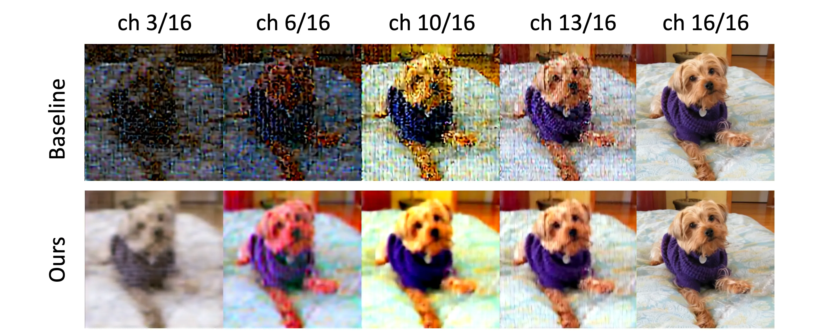
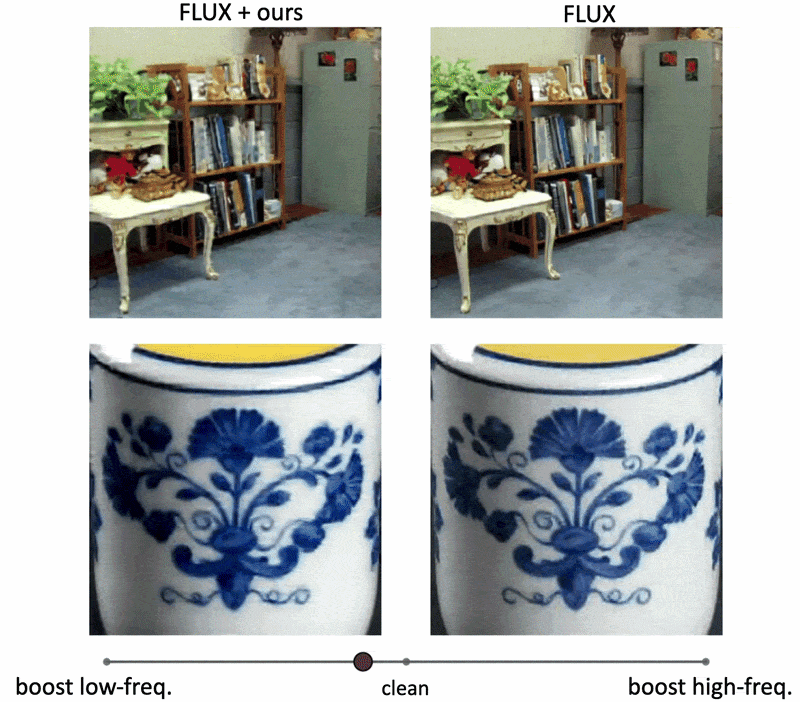
The visualization shows the progression as we unmask channels from low-to-high frequencies. Since low-frequency channels encode general layout of an image, you can see that using only three low-frequency-encoding channels already enables a pretty good image reconstruction. The derivation of the matrix lets us know which channel of the latent corresponds to low or high frequency, so we can deliberately mask out high-frequency-encoding channels to create progressive
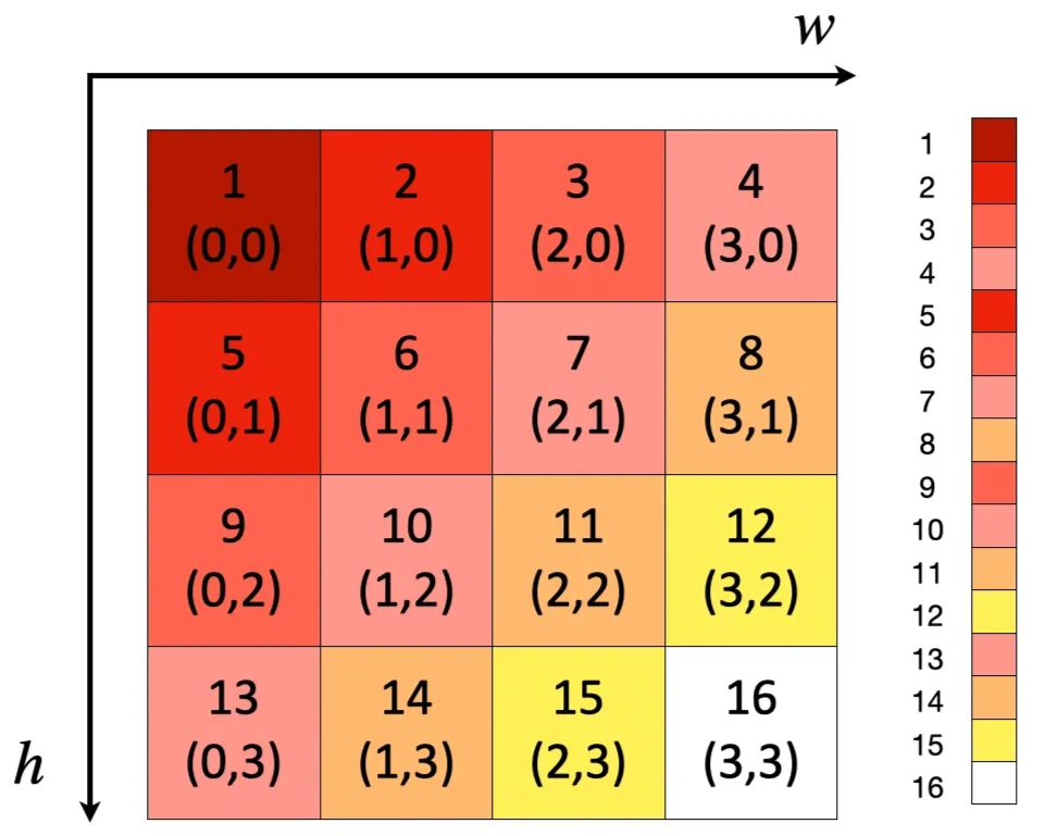
Toggle here to see which channel encodes which frequency bandThe matrix is defined as follows:
This leaves us to determine how we assign a set of 2D basis functions into a set of 1D indices:
We followed the most straightforward way to achieve this mapping: -first ordering, as illustrated in the following figure. The darker the color, the lower frequency a channel encodes.
Scaling a specific latent channel to boost a certain frequency component also yields similar results.
- Latent space’s effective rank decreased significantly.
The effective rank of the latent space is almost halved after regularization:
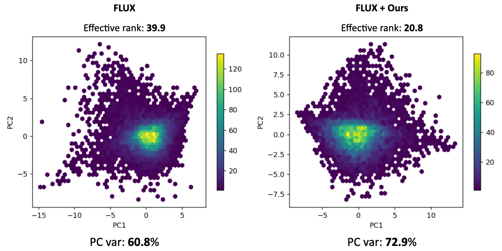
Above figure shows 10,000 images projected to the latent space, plotted using two PCA bases. The variance explained with PCA basis has increased from 60.8% to 72.9%, which also tells that it needs less orthogonal bases to fully explain the latent distribution.
🧐I personally believe that the rank has something to do with generation-friendliness.A lower rank means more redundancy among the latents, and that redundancy surfaces as statistical regularity — exactly the kind of structure a downstream generative model can lean on. In fact, there are a few studies claiming that latent distribution represented with fewer Gaussian modes and concentrated energy over few frequency bands is beneficial for generation.
I’ll be discussing this in future posts, hopefully.
Experiments: when trained on downstream generative models
When this regularization is applied to fine-tune tokenizers, it turned out that our assumptionsShow information for the linked content are half-wrong and half-right.
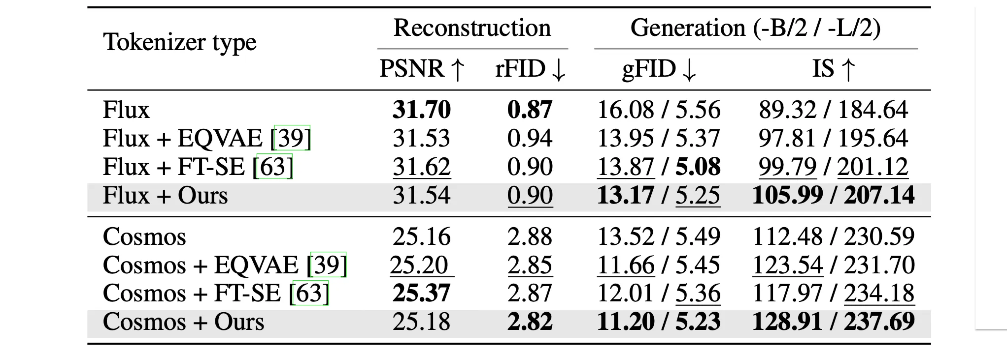
- Reconstruction quality is not enhanced. Although the regularization indeed guides the tokenizer’s encoder to divide the input image information in an orthogonal manner that enables compact compression (that’s how basis coefficients store the image information), it sacrifices the reconstruction training iterations by a factor of . Apparently, the tokenizers prefer to reconstruct images based on strategies created on their own, rather than being guided with compression function’s prior. Yet, it did not significantly harm the reconstruction performance either, even when compared to other regularizers that train the tokenizers to reconstruct images for the whole training iterations.
- Generation quality is enhanced. Our regularization does guide the latent feature’s channels to embed hierarchical nature of frequency components as we expected. Generation performance metrics indicate that the latent structures we enforced helped the downstream generative models to synthesize images. We also believe that this regularization encourage latent representations of images with similar spatial layouts to cluster together. Since such images naturally share similar low-frequency components, their corresponding latents are likely to agree on at least the low-frequency channels. This behavior may help shaping a smoother latent distribution. Intuitively, placing structurally similar images far apart in latent space introduces unnecessary complexity into the representation. By encouraging these latents to remain close, the model can organize the latent space more coherently, potentially making it easier to model and interpolate.
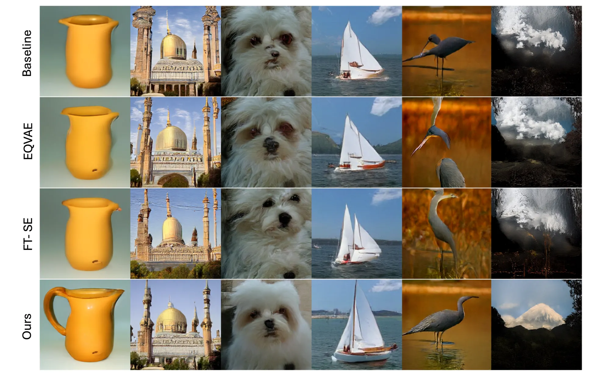
Generation examples from LightningDiT-B/2, using the Flux tokenizer
State-space regularization applied to image restoration
Regarding that state-space regularization produces features that separately encode different frequency bands, I thought it might benefit tasks like image restoration, such as denoising or super-resolution.
I did not dig these tasks deeper, but went through a prototypical attempt to see if our regularization method can potentially benefit image denoising (it actually is what generative model does, so it is worth trying!).
I chose one of the renowned image restoration model Restormer, and trained it for 30K iterations to denoise the real-world images with/without state-space regularization.
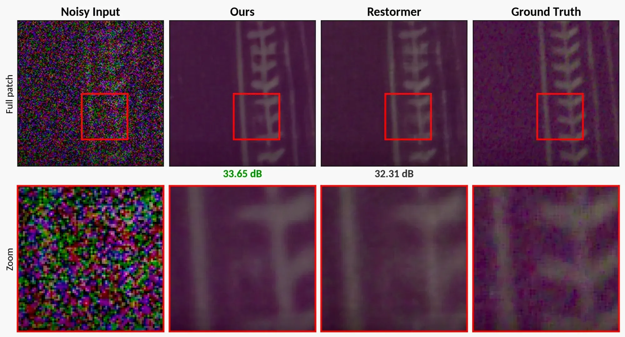
The effect was quite notable:
| Model | PSNR | SSIM |
|---|---|---|
| Restormer | 39.5803 | 0.9111 |
| w/ Ours | 39.8939 | 0.9128 |
I also attached the regularization to image super-resolution, but it did not seem to be as effective as it was in image denoising.
I initially considered exploring this direction further, but soon figured out that training image restoration models typically takes several days even for a single experiment. Given that this was only meant to be a proof-of-concept exploration, the required effort felt a bit too heavy, so I decided to leave it as an interesting future direction instead.
Closing thoughts

This series began with a simple goal: to come up with a 2-dimensional state-space model that makes more sense for visual data.
Interestingly, the journey did not end where I expected it to. The outcome was neither a new SSM module nor yet another Mamba-based vision backbone that achieves state-of-the-art results across benchmarks. Instead, it led me to a different way of applying SSMs to computer vision: through regularization.
While searching for a suitable application, the story took another unexpected deviation and drifted into the field of image tokenization—a topic that honestly deserves an entire series of its own. Apologies if some of the transitions felt abrupt or the explanations were a bit rushed 😅. Nevertheless, the resulting idea ended up making a surprisingly meaningful contribution: SSMs have rarely been used as a feature regularizer, nor have they explicitly been employed to improve frequency-awareness to enhance image generation and restoration.
What I found particularly exciting is that this exploration also uncovered some theoretically appealing connections. Along the way, we arrived at a mathematically well-defined structure for the matrix without explicitly engineering it to be diagonal, and stumbled upon a perspective that hints at a more generalized view of state-space models.
Perhaps this research was the most bent and crooked research I’ve ever done: I set out to solve one problem and end up finding something entirely different. But in fact, it was a very enjoyable journey, and I felt quite satisfied about the lessons I learned (although it is somewhat hard to be framed as a single paper in an organized manner 😂).
I hope some of the ideas in this series resonate with fellow SSM enthusiasts. If you have thoughts, questions, or completely different interpretations, I'd love to hear them in the comments.
With that, this concludes the "Towards 2-Dimensional State-Space Models" series.
Next time, I'll return with something a little more casual: a post about my time in Brazil while attending ICLR 2026! Tchau 🤙🏼