Towards 2-Dimensional State-Space Models (2): WHippo

This post continues from the previous post: Towards 2-Dimensional State-Space Models (1): Intro.

Once we accept the separation of the sequence construction order $t$ and the spatial coordinates $(h,w)$ , we can consider wide range of image transformations that align much better with inherent image properties.

Few transformations that would come to your mind would be:

Then, what’s next? Can we construct SSMs on this?

A generalized view of SSMs

I spent quite a lot of time thinking about ways to derive a valid SSM on this concept. I started from HiPPO (Gu et al., NeurIPS 2020), since that’s where the 1D SSMs are built upon.

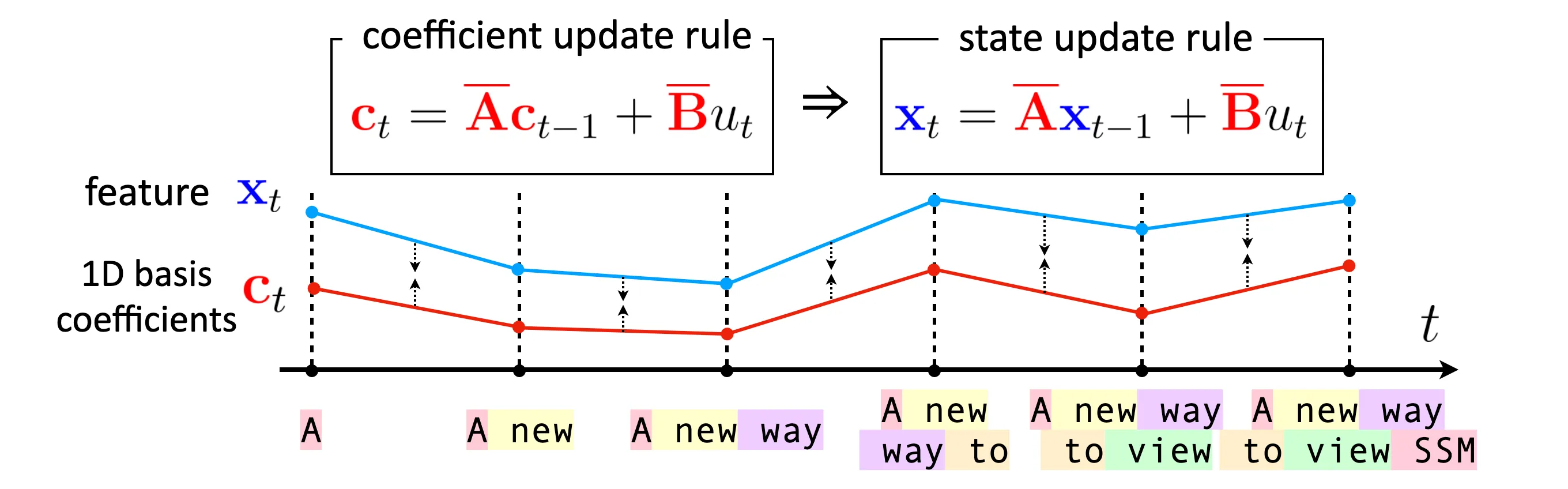
HiPPO derives how orthogonal polynomial coefficients change every time a new token is appended to the end of the input sequence.

To briefly explain, HiPPO manually derived the dynamics of orthogonal polynomial coefficients that reflects the newly added token $u_t$ , and let the RNN’s hidden update follow this dynamics, as described in the figure above. I provide you more detailed explanation in my previous post.

At the end, I figured that SSMs are implicitly nudged to follow designated compression function (or basis projection, for mathematical ease) that we choose in the first place. Let me explain this in a more principled way.

In my opinion, the mechanisms of existing SSMs can be characterized by two components:

a compression function $\mathbf{c}: \bigcup\limits_{L\in \mathbb{N}_{\scriptscriptstyle{\geq N}}} \mathbb{R}^{L} \rightarrow \mathbb{R}^{N}$ ,
an input transformation $\theta : \mathbf{I}_{t-1} \mapsto \mathbf{I}_{t}$ , where $\mathbf{I}_{t}$ denotes the input at time $t$ .

With this setup, we can explain pretty much of the existing SSMs, either 1D or 2D.

For example, HiPPO chose the compression function $\mathbf{c}(\cdot)$ as a projection using 1D orthogonal polynomials, while choosing the input transformation $\theta : \mathbf{I}_{t-1} \mapsto \mathbf{I}_{t}$ as a concatenation of the $t$ -th token next to the 1D input at time $t-1$ .

Letting $\mathbf{c}(\cdot)$ be the projection using 2D orthogonal polynomials and $\{\mathbf{I}_t\}$ be the corner-based construction using 2-dimensional sweeping will coincide with the formulation introduced in S4ND or 2D-SSM.

In fact, we can regard that the hidden states of SSMs are trained to resemble the behavior of compression function $\mathbf{c}(\cdot)$ in an indirect way; by mimicking its dynamics $\frac{\mathrm{d}}{\mathrm{d}t}\mathbf{c}(\mathbf{I}_t)$ on the predefined input transformation $\theta$ , rather than mimicking its actual outputs.

This somehow explains where the compactness—the well-known ability of SSMs—emerges from: it may be due to its inherent design pushing the hidden state to resemble the compression function $\mathbf{c}(\cdot)$ . To step a little further, if you choose a typical basis function projection as $\mathbf{c}(\cdot)$ , you can expect the hidden state to capture spectral components of the input, as one of the properties that a lot of basis projections have is the decomposition of the input into spectral components. With this approach, you can distill favorable properties of $\mathbf{c}(\cdot)$ to the hidden state, which has been an effective strategy for SSMs.

Thus, if we choose a combination of compression function and input transformation $\bigl(\mathbf{c}(\cdot), \theta(\cdot)\bigr)$ and enforce a feature to follow the update rule induced by $\mathbf{c}(\mathbf{I}_{t-1}) \mapsto \mathbf{c}(\mathbf{I}_{t})$ , we can come up with a novel SSM formulation that inherits the SSM’s core strategy.

WHippo: finding a good $\bigl(\mathbf{c}(\cdot), \theta(\cdot)\bigr)$ combination

<Vision Mamba>
\theta(\cdot) : 1D scanning
\mathbf{c}(\cdot) : 1D OP projection — <Vision Mamba>
$\theta(\cdot)$ : 1D scanning
$\mathbf{c}(\cdot)$ : 1D OP projection

<S4ND, 2D-SSM>
\theta(\cdot) : 2D scanning
\mathbf{c}(\cdot) : 2D OP projection — <S4ND, 2D-SSM>
$\theta(\cdot)$ : 2D scanning
$\mathbf{c}(\cdot)$ : 2D OP projection

<Ours ( WHippo )>
\theta(\cdot) : Gaussian blurring
\mathbf{c}(\cdot) : 2D OP projection — <Ours (*WHippo*)>
$\theta(\cdot)$ : Gaussian blurring
$\mathbf{c}(\cdot)$ : 2D OP projection

The illustration above shows the choice of $\theta(\cdot)$ with designated compression function $\mathbf{c}(\cdot)$ .

One thing to note when choosing $\mathbf{c}(\cdot)$ and $\theta(\cdot)$ is to ensure that the update $\mathbf{c}(\mathbf{I}_{t-1}) \mapsto \mathbf{c}(\mathbf{I}_t)$ is tractable: the dynamics of compressed representation $\mathbf{c}(\cdot)$ must be computable without having to decompress the input. This is related to the derive-ability of the derivative $\frac{\mathrm{d}\mathbf{c}(\mathbf{I}_t)}{\mathrm{d}t}$ , and explains why it is convenient to use basis projection as the compression function $\mathbf{c}(\cdot)$ ; basis projection is often smooth and differentiable, compared to other compression formats such as PNG or Huffman Coding.

WHippo chooses \mathbf{c}(\cdot) as 2D basis projection, and \theta(\cdot) as Gaussian blurring — WHippo chooses $\mathbf{c}(\cdot)$ as 2D basis projection, and $\theta(\cdot)$ as Gaussian blurring

My friend Jaemin and I found that choosing $\mathbf{c}(\cdot)$ as 2D orthogonal polynomial basis projection and $\theta(\cdot)$ as Gaussian blurring results in a quite simple update rule, and we name this framework, WHippo.

Why named WHippo?

The biological classification of hippo is called Whippomorpha, which is a class of mammals that includes whales and hippos. So, Whippo can be viewed as a superclass (or generalization) of hippo.
This idea is a continuation of HiPPO (NeurIPS 2020), which was the starting point of the state-space model, and we are trying to extend HiPPO to 2D, which previously only worked in 1D. Therefore, our HiPPO has spatial dimensions (Width, Height).

Why Gaussian blurring?

TL;DR, the Gaussian kernel provides a lot of really nice properties that align with our visual perception process, and reflects inherent property of natural images as well.

Scale-space theory: A basic tool for analyzing structures at different scales (Tony Lindeberg, 1994; Journal of Applied Statistics) talks about scale-space in images.

Research on finding better ways to analyze a given input at different scales is one of the oldest challenges in computer vision, and this paper is one of the classic theories on this subject. Here they study blurring techniques that allow us to obtain good scale representations and introduce the resulting method.

... This chapter gives a tutorial review of a special type of multi-scale representation, linear scale-space representation, which has been developed by the computer vision community in order to handle image structures at different scales in a consistent manner...
The main result we will arrive at is that if rather general conditions are posed on the types of computations that are to be performed at the first stages of visual processing, then the Gaussian kernel and its derivatives are singled out as the only possible smoothing kernels.

In our case, the Gaussian kernel provides a number of good properties in other means as well. The Gaussian kernel is defined in a continuous manner, is deterministic, and preserves linearity (applying two Gaussian kernels of $\sigma_1$ and $\sigma_2$ results in applying a single Gaussian kernel of $(\sigma_1 + \sigma_2)$ ). This largely helps our derivation of $\frac{\mathrm{d}\mathbf{c}(\mathbf{I}_t)}{\mathrm{d}t}$ later.

Derivation of the WHippo update rule

Hence, our next step would be to derive the update rule $\mathbf{c}(\mathbf{I}_{t-1}) \mapsto \mathbf{c}(\mathbf{I}_{t})$ based on the chosen $\bigl(\mathbf{c}(\cdot), \theta(\cdot)\bigr)$ .

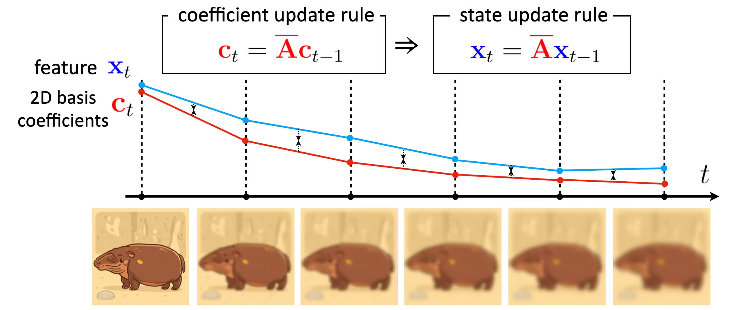
The figure aboveShow information for the linked content already spoils how the update rule looks like: it actually ends up inducing a pretty simple rule:

\begin{align} \frac{\mathrm{d}\mathbf{c}_t}{\mathrm{d}t} = \mathbf{A}\mathbf{c}_t \quad \xRightarrow[]{\text{discretize (e.g., euler)}} \quad \mathbf{c}_{t+1} \ &= (\mathbf{1}+\Delta \mathbf{A})\mathbf{c}_t \\ & := \overline{\mathbf{A}}\mathbf{c}_t \nonumber \end{align}

with a structured matrix $\mathbf{A}$ .

Below I provide the derivation process of the update rule. Hopefully, its derivation process is not as hard as that of HiPPO’s.

Let’s assume an image with only one channel $\mathbf{I} \in \mathbb{R}^{H \times W}$ and derive the expression.
(although the illustrations show an RGB image)

Here, we assume the image $\mathbf{I}$ as a surface function $\mathbf{I}(x,y)$ rather than a set of discrete points, which makes our formulation perfectly analogous to the original 1D SSM’s derivation.

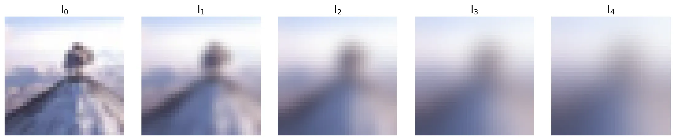
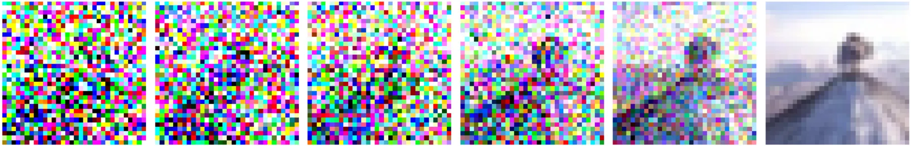
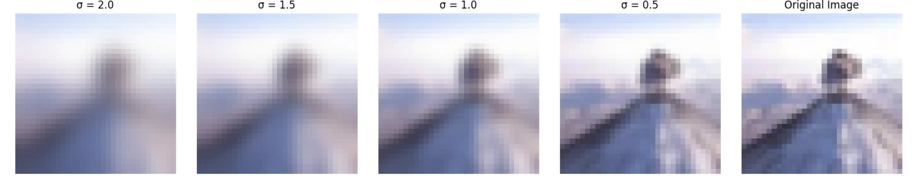
Let a continuous sequence of images with increasingly blurred images be $\{ \mathbf{I}_t\}_{t \in [0, T]}$ ( $\mathbf{I} = \mathbf{I}_0$ ), where the Gaussian kernel $G_t$ applied at $t$ -th timestep is

G_t(x,y) = \frac{1}{2\pi t}\exp(-\frac{x^2 + y^2}{2t}).

Then the image $\mathbf{I}_t$ can be viewed $\mathbf{I}_0 *G_t$ , where $*$ is the convolution operation. We can obtain the coefficients $\mathbf{c}(t) = \begin{bmatrix} c_1(t) & c_2(t) & \cdots &\ c_{HW}(t) \end{bmatrix}^\top$ corresponding to the 2D basis functions $\{\phi_k\}_{k=1}^{HW}$ by projecting an image onto the basis functions:

c_k (t) = \langle G_t * \mathbf{I}, \phi_k \rangle = \iint_{[0,H]\times [0,W]}(G_t * \mathbf{I})(x,y)\cdot \phi_k(x,y)\mathrm{d}y\mathrm{d}x.

We are interested in the dynamics of $c_k(t)$ with respect to $t$ , so differentiating both sides with respect to $t$ gives:

\begin{align}\frac{\mathrm{d}c_k(t)}{\mathrm{d}t} = \frac{\mathrm{d}}{\mathrm{d}t}\langle G_t * \mathbf{I}, \phi_k \rangle = \Bigl\langle \frac{\partial}{\partial t}(G_t * \mathbf{I}), \phi_k \Bigr\rangle. \end{align}

Note that convolution with a Gaussian filter is a well known solution of heat equations.

What does this mean?

Assume a trivariate function $T(x,y,t)$ , which models how the temperature at each $(x,y)$ coordinate (on $[0,H] \times [0,W]$ as defined above) changes over time, then the PDE Heat equation (or, diffusion equation) describes the amount of temperature change at each point as follows:

\frac{\partial T}{\partial t}= \alpha \Bigl(\frac{\partial^2 T}{\partial x^2} + \frac{\partial^2 T}{\partial y^2}\Bigr) := \alpha \nabla^2 T.

If $T(x,y,0)$ , the temperature distribution at time $t=0$ (initial value condition), and derivatives at $(x,y)$ boundaries, $\frac{\partial T}{\partial x}|_{x\in \{0, H\}}$ , $\frac{\partial T}{\partial y}|_{y\in \{0, W\}}$ (boundary conditions; we usually let them be zero, following standard Neumann boundary condition) are given, we can find the solution of the above equation. The known solution is $u(x,y,t):=G_t * \mathbf{I}$ . More precisely, it is satisfied when the standard deviation of the Gaussian filter $G_t$ is $\sqrt{2\alpha t}$ .

In other words, if we consider the initial value $\mathbf{I}_0$ in the image sequence aboveShow information for the linked content to be the temperature rather than the pixel intensity, then the pixels $\mathbf{I}_t$ becomes equivalent to representing the temperature after $t$ .

$(G_t * \mathbf{I})$ is the solution to the heat equation $\frac{\partial T}{\partial t}= \frac{1}{2} \Bigl(\frac{\partial^2 T}{\partial x^2} + \frac{\partial^2 T}{\partial y^2}\Bigr) := \frac{1}{2} \nabla^2 T$ , so the partial differential term appearing in (2) can be summarized as follows:

\Bigl\langle \frac{\partial}{\partial t}(G_t * \mathbf{I}), \phi_k \Bigr\rangle = \Bigl\langle \frac{1}{2}\nabla^2(G_t * \mathbf{I}), \phi_k \Bigr\rangle.

On the other hand, before computing the above, we can reorganize terms cleaner if we first represent the image $(G_t * \mathbf{I})$ ) of each step as a sum of basis functions $\phi_k$ . Since we already have defined the coefficients $\mathbf{c}(t)$ of the basis functions, we can easily use them to express $(G_t *\mathbf{I})(x,y) = \mathbf{c}(t)^T \mathbf{\phi}(x,y)= \sum_{i=1}^{HW}c_i(t)\phi_i(x,y)$ and substitute them:

\begin{align*} \Bigl\langle \frac{1}{2}\nabla^2(G_t * \mathbf{I}), \phi_k \Bigr\rangle &= \frac{1}{2} \Bigl\langle \sum_{i=1}^{HW}c_i(t)\nabla^2\phi_i, \phi_k \Bigr\rangle \\ &= \frac{1}{2} \sum_{i=1}^{HW}c_i(t) \Bigl\langle \nabla^2\phi_i, \phi_k \Bigr\rangle. \end{align*}

From here, the derivation can either be easier or harder depending on which basis function $\phi$ you choose.

In general, good basis functions assume orthogonal properties, so the basis function that allows $\nabla^2 \phi_k$ to be expressed with $\phi_k$ will be the easiest to derive.
(For example, in the case of Fourier, $\nabla^2 \phi_k$ is a scaled $\phi_k$ term, so we can expect a very clean expression!)

The final expression:

\frac{\mathrm{d}c_k(t)}{\mathrm{d}t} = \frac{1}{2} \sum_{i=1}^{HW}c_i(t) \Bigl\langle \nabla^2\phi_i, \phi_k \Bigr\rangle \qquad ---- \quad (*)

The good news is that we actually already have an expression that looks like a simple form of the SSM. Since the change in $c_k$ is expressed as a linear combination of different $c_k$ ’s, this can be understood as a matrix operation:

\begin{align} \frac{\mathrm{d}}{\mathrm{d}t}\mathbf{c}(t) &= \frac{1}{2} \begin{bmatrix} \langle \nabla^2\phi_1, \phi_1 \rangle & \langle \nabla^2\phi_1, \phi_2 \rangle & \cdots & \langle \nabla^2\phi_{1}, \phi_{HW} \rangle \\ \langle \nabla^2\phi_2, \phi_1 \rangle & \langle \nabla^2\phi_2, \phi_2 \rangle & \cdots & \langle \nabla^2\phi_{2}, \phi_{HW} \rangle \\ \vdots & \vdots & \ddots & \vdots \\ \langle \nabla^2\phi_{HW}, \phi_1 \rangle & \langle \nabla^2\phi_{HW}, \phi_2 \rangle & \cdots & \langle \nabla^2\phi_{HW}, \phi_{HW} \rangle \\ \end{bmatrix} \mathbf{c}(t) \nonumber \\ &:= \mathbf{A}\mathbf{c}(t). \nonumber \end{align}

The WHippo matrix $\mathbf{A}$

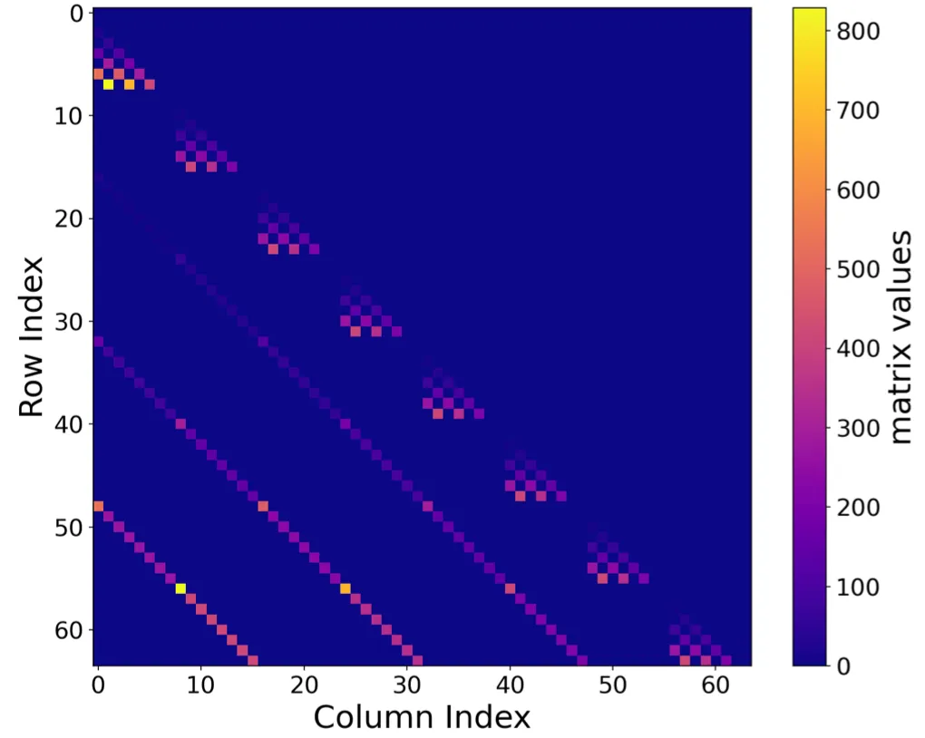
The structure of the matrix $\mathbf{A}$ is solely dependent on the choice of the 2D basis function $\phi$ .

I’ll skip the derivation of $\mathbf{A}$ matrices of different bases, but I think it is worth sharing how they look like. Below are figures of those matrices, and you can see their sparse structures.

\mathbf{A} of 2D Fourier bases — $\mathbf{A}$ of 2D Fourier bases

\mathbf{A} of 2D Legendre polynomial bases — $\mathbf{A}$ of 2D Legendre polynomial bases

\mathbf{A} of 2D Chebyshev polynomial bases — $\mathbf{A}$ of 2D Chebyshev polynomial bases

\mathbf{A} of 2D Hermite polynomial bases. Due to its exponential values, log values are displayed. Zero values marked white. — $\mathbf{A}$ of 2D Hermite polynomial bases. Due to its exponential values, log values are displayed. Zero values marked white.

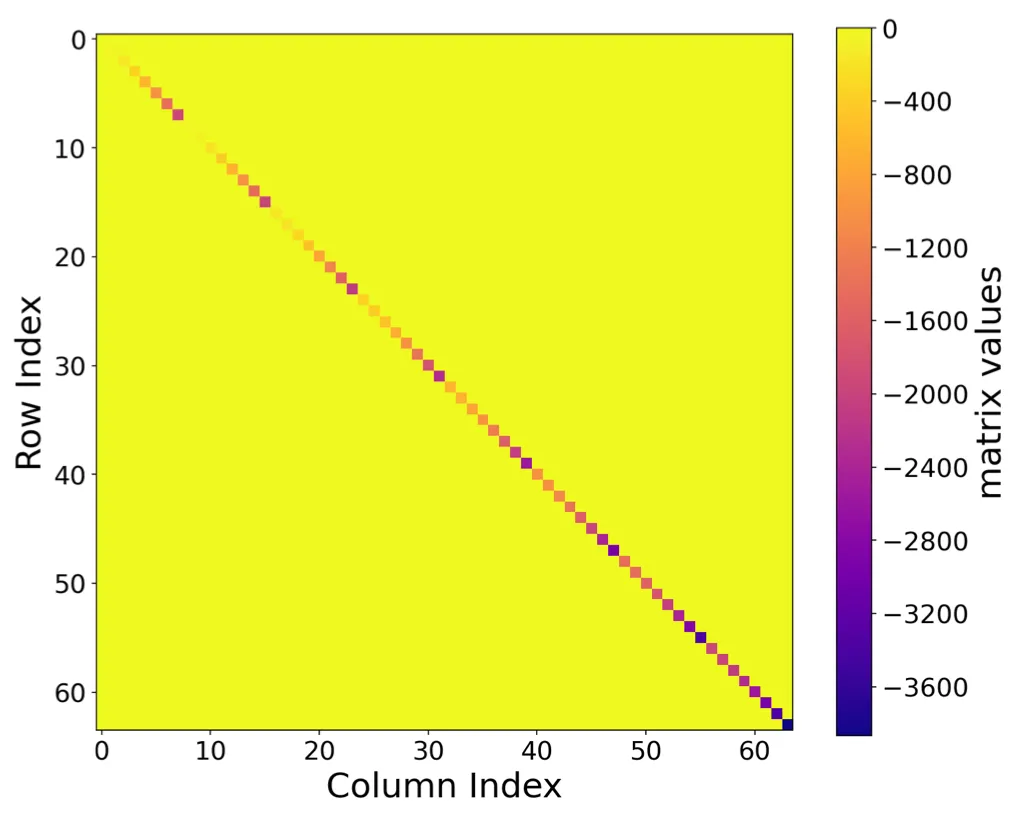
One particularly interesting observation is that choosing Fourier bases projection as $\mathbf{c}(\cdot)$ naturally yields a diagonal matrix $\mathbf{A}$ , which has long been preferred in 1D SSMs due to its simplicity of computing matrix powers. Regarding that numerous studies have been devoted to simplifying S4’s diagonal-plus-low-rank (DPLR) formulation by removing the low-rank correction in order to enjoy the efficient and simplified nature of diagonal matrix, it is quite intriguing that a diagonal form of $\mathbf{A}$ emerges here for free: we do not rely on any approximation, nor do we need to empirically justify whether the resulting parameterization is expressive enough.

Little caveats from the diagonal WHippo $\mathbf{A}$

Looking into details of Fourier-based diagonal WHippo $\mathbf{A}$ tells us some more interesting facts.

The $k$ -th diagonal values of $\mathbf{A} \in \mathbb{R}^{HW \times HW}$ is

\begin{equation} \lambda_k = -2WH\pi^2\bigl( \frac{w^2}{W^2} + \frac{h^2}{H^2} \bigr), \end{equation}

where $w = (k-1) \bmod W$ and $h=\lfloor\frac{k-1}{W}\rfloor$ .

To provide a concrete view, I visualized the matrix where $(H,W) = (4,5)$ :

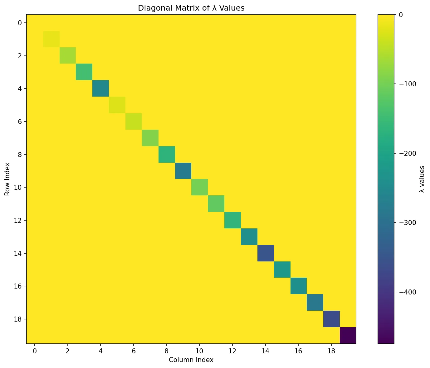
Here, we observed two caveats that are worth to discuss.

Every $\lambda_k$ is a negative real value, as S4D and SaShiMi propose:

(from S4D)
Note that the kernel $K(t) = \mathbf{C}e^{t\mathbf{A}}\mathbf{B}$ blows up to $\infty$ as $t \to \infty$ if $\mathbf{A}$ has any eigenvalues with positive real part. Goel et al. found that this is a serious constraint that affects the stability of the model, especially when using the SSM autoregressively. They propose to force the real part of $\mathbf{A}$ to be negative, also known as the left-half plane condition in classical controls, by parameterizing the real part inside an exponential function $\mathbf{A}=−\exp(A_\textrm{Re}) + i·A_\textrm{Im}$ .

The main reason for $\lambda$ s being parameterized negative was for training stability. The diagonal WHippo matrix already provides such a well-initialized $\mathbf{A}$ , without having to engineer this property into the model.
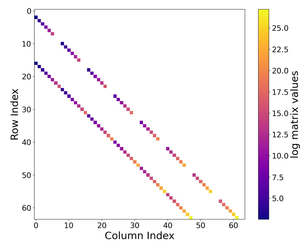
It resembles how Mamba’s diagonal matrix $\mathbf{A}$ is initialized… but in two dimensions!
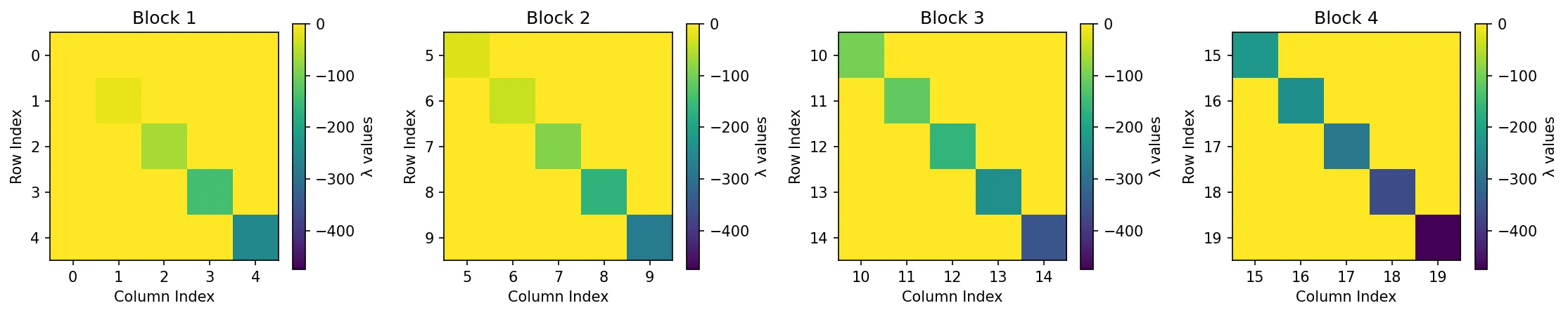
When we group diagonal elements into $(W,W)$ -sized blocks, we can see analogous evolutions across the blocks. According to Eq. (3)Show information for the linked content, the values grow in a squared scale across both dimensions $h$ and $w$ .
We strongly believe that there is a connection between ours and S4ND, as this way of multi-dimensional initialization resembles how S4ND constructs SSM kernels using cross-product.
Comparing this to the Mamba $\mathbf{A}$ ’s (or, S4D-Real’s) initialization, we can find an interesting resemblance again:
Mamba initializes its diagonal elements by assigning incrementally decreasing negative integers: $-1, -2, -3, \ldots$ , and each block of Show information for the linked content $\mathbf{A}$ shows the similar tendency. If we really do want to stick to the Mamba’s legacy, one might be able to do so by initializing the first block matrix’s diagonal elements as $\{-1, -2, -3, \ldots \}$ and the next block’s as $\{-2, -3, -4, \ldots \}$ , yielding a natural multi-dimensional generalization.

🔎

The tradition of $-1$ increment is derived from setting $\mathbf{c(\cdot})$ as legendre polynomial in the previous studies. We also observed that deriving the matrix from legendre polynomial gives a matrix with a very stable scale, linear to the matrix size $HW$ : see Legendre Show information for the linked content $\mathbf{A}$ , and you can observe that it is the only case where the matrix values are on a pleasant scale. Other than that, we could not find more meaningful insights yet.

So, what’s next? Any use of this?

Now we derived a novel 2D SSM formulation that is more natural in terms of image processing.

Then, how can this be implemented in neural network training?

I’ll explain its intriguing usage in the next post. To tease a little bit, there was an unexpected property that this framework provides to diffusion modeling!

A generalized view of SSMs

WHippo: finding a good (c(⋅),θ(⋅))\bigl(\mathbf{c}(\cdot), \theta(\cdot)\bigr)(c(⋅),θ(⋅)) combination

Derivation of the WHippo update rule

What does this mean?

The WHippo matrix A\mathbf{A}A

Little caveats from the diagonal WHippo A\mathbf{A}A

So, what’s next? Any use of this?

WHippo: finding a good $\bigl(\mathbf{c}(\cdot), \theta(\cdot)\bigr)$ combination

The WHippo matrix $\mathbf{A}$

Little caveats from the diagonal WHippo $\mathbf{A}$