How Compressionists Think (3): Variational Autoencoders are Compressors

This post continues from the previous post: How Compressionists Think (2).

ARC-AGI Without Pretraining

ARC-AGI Without Pretraining is a paper from Albert Gu’s Goomba lab.

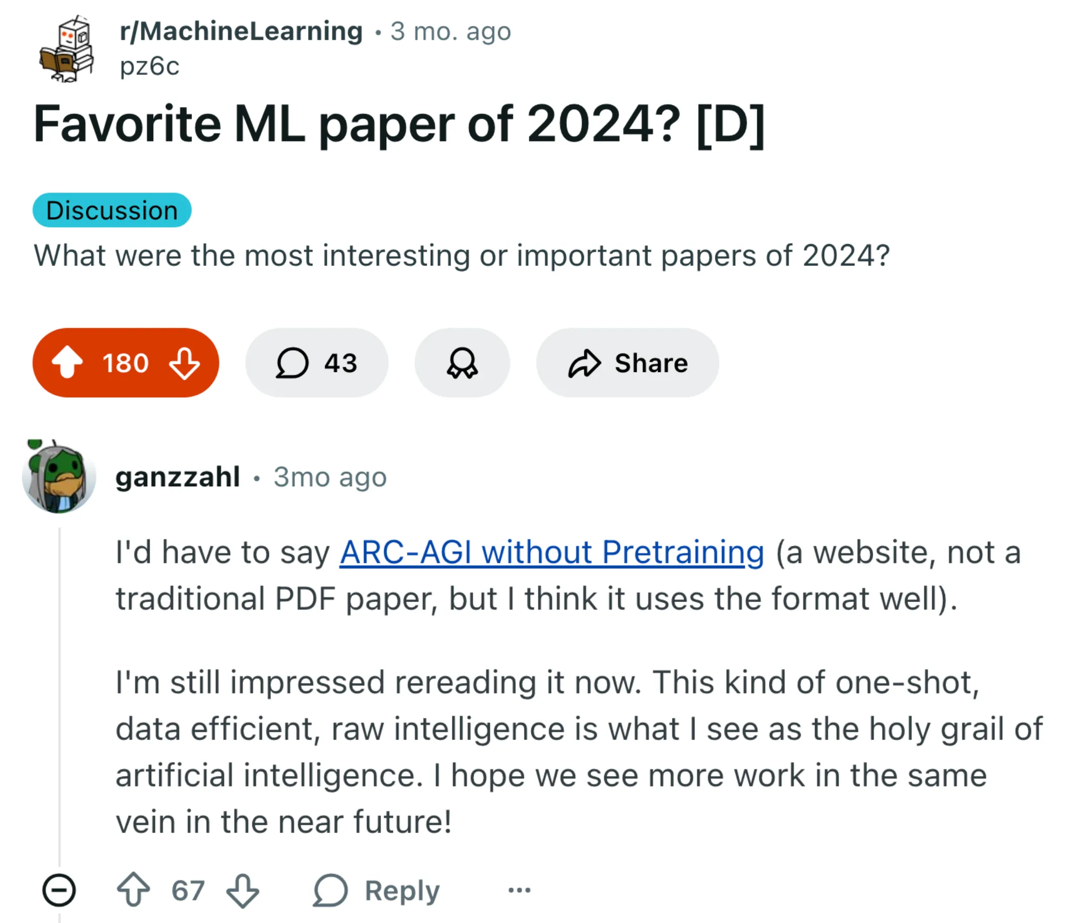
I encountered this paper on this reddit post, where people upvoted for their favorite ML paper of 2024.

Apparently, people were fascinated by how the paper managed to solve puzzles using nothing but a pure compression objective, without ever being trained on a massive dataset.

Let me briefly walk you through what this paper is about, and how it connects the idea of compression to generation model — not with the text this time, but with images.

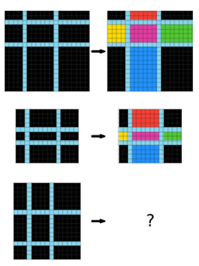
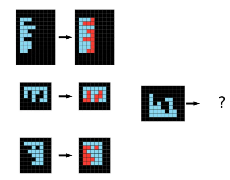
This paper aims to solve puzzles from ARC-AGI 1 which in general looks like this:

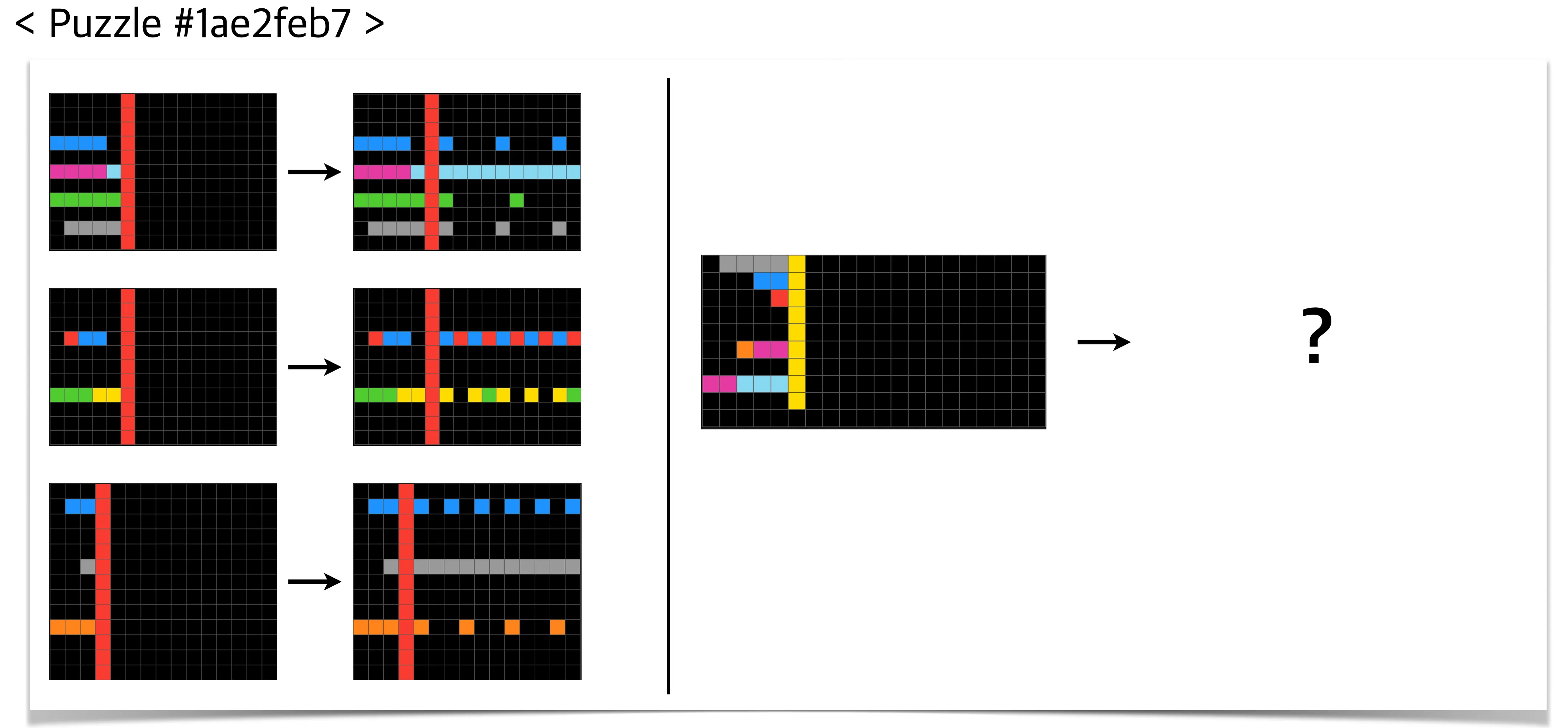
puzzle answer

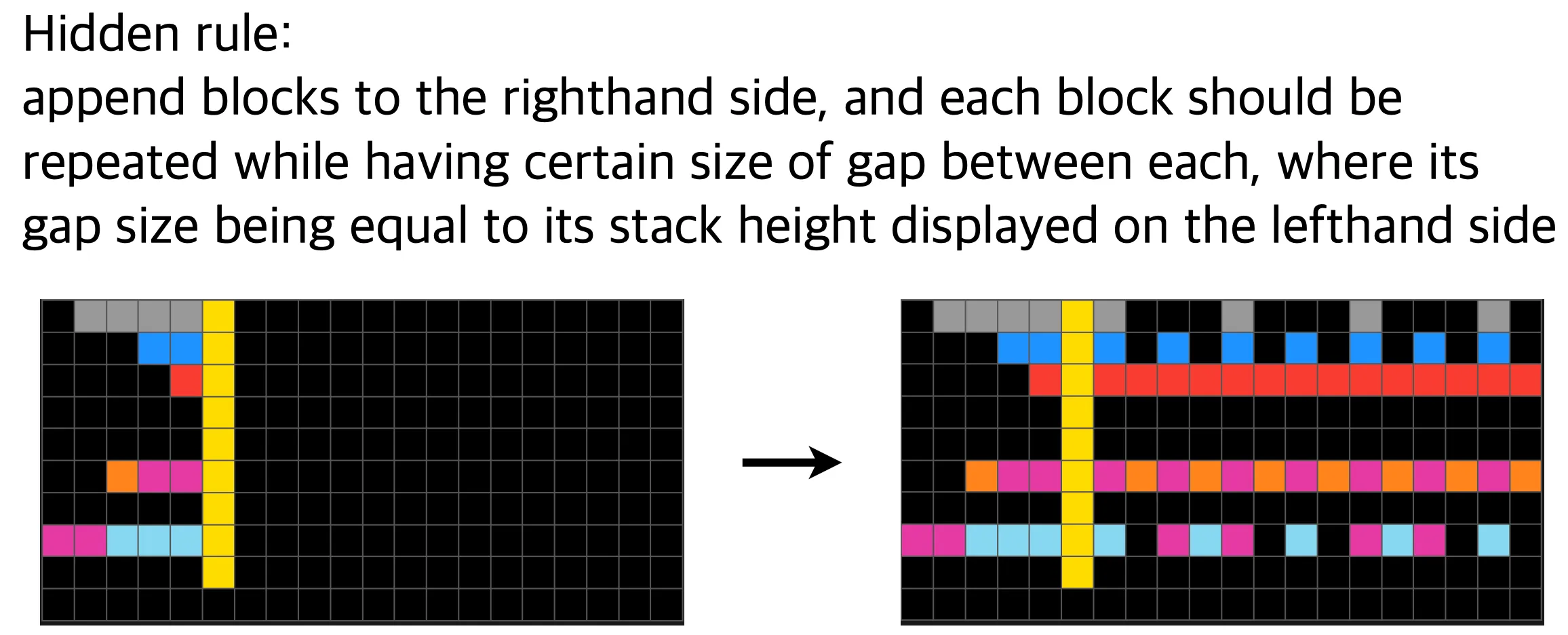
It gives you several puzzles with answers to let you infer the hidden rule, and you are asked to determine the size of the answer puzzle as well as each pixel’s color.

(from the original blog post)
The puzzles are designed so that humans can reasonably find the answer, but machines should have more difficulty. The average human can solve 76.2% of the training set, and a human expert can solve 98.5%.

The way authors dealt with the problem was: let’s train a generative model that is likely to generate given puzzle-answer pairs — but under the compression constraint; this generative model should be expressed with least bits. It shares a similar idea with code golfing problem, which is mentioned earlier hereShow information for the linked content.

Since a generative model approximates a distribution, this can be also understood as finding the simplest distribution that explains the current phenomena; which aligns with the well-known philosophy Occam’s razor.

Hence, the authors expected the model would implicitly go through the process of finding patterns of the given problems and eventually end up finding the shortest explanation to describe the hidden rules, if given a proper compression objective.

The “proper” compression objectives that the authors come up with are illustrated in the figure below: reconstruction loss, regularization loss, and KL loss.

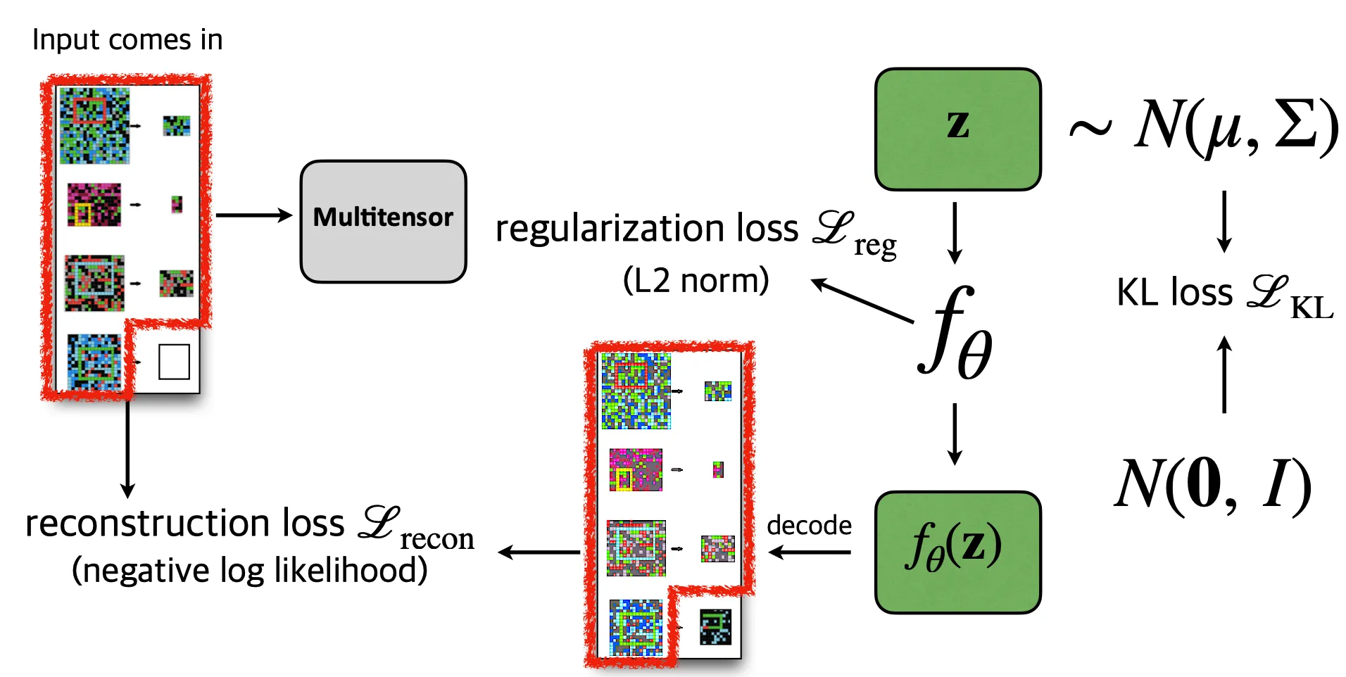
Let me briefly explain how this model works.

That’s pretty much it.

The unknown part, is filled with whatever the model returns for that part, and it surprisingly well approximates the answer!

That seems not really trivial, right?

So, how do these three losses—reconstruction loss, regularization loss, KL loss—enable such non-trivial phenomenon? Why are these even translated to “compression” objective?

Let’s see how authors come up with these losses.

ARC-AGI as Code golfing problem

Code golfing problem is a type of computer programming competition, where you need to create a minimal code that solves the given problem. The primary scoring criterion is based on its code length; above all the concerns, all that matters is the length of the code itself.

It partially stems from the idea of Jorma Rissanen’s Minimum Description Length (MDL) principle:

(Quoted from here)
A criterion for estimation of parameters (…) has been derived from the single and natural principle: minimize the number of bus it takes to write down the observed sequence.

Note that MDL offers a sound way to compress a potentially infinite length of data; for example, a reasonable way to compress the following infinite sequence:

$$1, 4, 9, 16, 25, 36, 49,64,\ldots$$

would be to describe the sequence with least characters, such as $\{t^2\}_{t=0}^{\infty}$ or “a sequence of squared non-zero integers in increasing order”, rather than a traditional compression technique that takes all the inputs to create a compressed form.

ARC-AGI problem can also be viewed from this perspective:

Under this compression-like objective, compressionists expect the ARC-AGI-generating program code to understand the rule behind the given puzzle in order to achieve minimal code length possible.

Authors further give some constraints on this “program code” to well-define the problem: it should be entirely self-contained, receive no inputs, and print out the entire ARC-AGI dataset of puzzles with any solutions filled in.

The resulting design of the program $P$ involves three components:

Consequently, what program $P$ does is to forward pass $f_\theta(\mathbf{z})+ \epsilon$ to produce puzzles and answers in the ARC-AGI dataset.
(Technically it should be $\text{decode}(f_\theta(\mathbf{z}) )+ \epsilon$ if it happens in multitensor latent space)

Then this leads to a natural question.

How should we define and measure the length of the program?

Since the program $P$ consists of $\theta$, $\mathbf{z}$, and $\epsilon$, authors came up with an idea of turning these into a form of bitstream: $s_\theta$, $s_\mathbf{z}$, $s_\epsilon$, and measure their respective length.

Turning $\epsilon$ into a bitstream $s_\epsilon$

The output correction $\epsilon$ can be understood as the error between the estimation $f_\theta(\mathbf{z})$ and the actual puzzle. Having a zero-valued $\epsilon$ should be the ideal case, and thus it is natural to have a bitstream $s_\epsilon$ having shorter length when the error is small.

What authors chose for bitstream conversion was “arithmetic coding”, a classical lossless compression method that turns data into a bitstream based on the data’s entropy. Specifically, the bitstream conversion using arithmetic coding requires a probability density function $p$ of the data they try to compress, which significantly affects the resulting bitstream’s length. In general, we cannot really know $p$ and one instead uses its estimation $\hat{p}$, which leads to a suboptimal bitstream length compared to the ground-truth $p$.

In fact, the length of the compressed bitstream $\text{len}(s_\epsilon)$ is proportional to $d(p, \hat{p})$, where $d$ is a distance measure between two distributions. The most natural choice for $d$ is cross-entropy loss between $p$ and $\hat{p}$, which can also be minimized by the cross-entropy loss between the estimated puzzle $f_\theta(\mathbf{z})$ and the actual puzzle.

Consequently, $\text{len}(s_\epsilon)$ corresponds to the recontruction loss $\mathcal{L}_{\text{recon}}$ in this figureShow information for the linked content.

Turning $(\theta, \mathbf{z})$ into bitstreams $(s_\theta, s_\mathbf{z})$

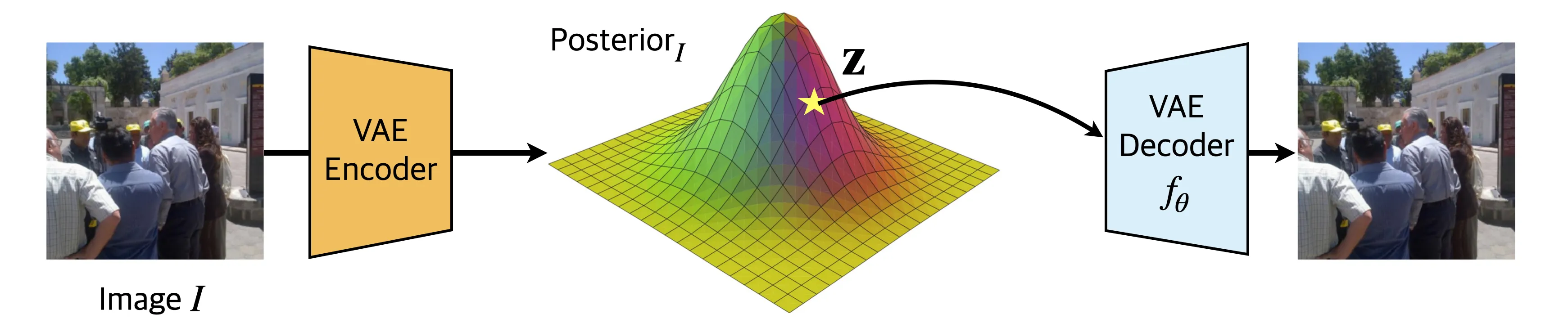
The authors borrowed ways to bitstream-ize $\theta$ and $\mathbf{z}$ from the paper REC, which tries to compress an image using variational autoencoders (VAEs).

Let’s say this VAE is trained under the following objective:

REC (and many other VAE-based image compression method) share a simple core idea to represent an image $I$ with fewer bits:

• Image $I$ is mapped to a latent variable $\mathbf{z}$, which is supposed to lie on latent distribution $q(\mathbf{z}|I)$. Depending on the strength of the KL loss, it should resemble the known distribution $p(\mathbf{z})$ (we usually set this prior as $\mathcal{N(0, \mathbf{I})}$)
• Deterministic decoder $f_\theta$ maps the latent $\mathbf{z}$ back to the pixel space.
• For this to function as compression, $\theta$ and $\mathbf{z}$—the ingredients to reconstruct the image (via $f_\theta(\mathbf{z})$)—should be representable with fewer bits than the original image $I$. This highly depends on the entropy of $\mathbf{z}$ and the weight $\theta$: the more entropy they have (i.e., the less regularities they contain, see hereShow information for the linked content), the more bits are required to represent them in a compressed representation.

Hence, the VAE-based image compression methods often utilize objectives that minimize the entropy of $\mathbf{z}$ and $\theta$, and this is equivalent to minimizing the bitstream $s_{\mathbf{z}}$ and $s_{\theta}$.

REC showed the followings:

• $\begin{aligned} \mathbb{E}[\text{len}(s_\theta)] = KL(p_\theta \Vert q_\theta) = \mathbb{E}_{\theta \sim p\theta} [\log (p_\theta(\theta) / q_\theta(\theta))] &\approx \lambda \lVert \theta \rVert^2 + \text{const} \end{aligned}$,
  where $q_\theta = N(0, I/2)$.
• $\mathbb{E}[\text{len}(s_\mathbf{z})] = KL(p_\mathbf{z} \lVert q_\mathbf{z}) = \mathbb{E}_{\mathbf{z} \sim p_\mathbf{z}} [\log (p_\mathbf{z}(\mathbf{z}) / q_\mathbf{z}(\mathbf{z}))],$
  where $q_\mathbf{z} = N(0, I)$.

Note that $\mathbf{z}$ is a latent variable while $\theta$ is a network parameter, which is why you cannot really handle $\mathbf{z}$ like the case of $\theta$.

The above implies that minimizing $\text{len}(s_\theta)$ corresponds to minimizing weight decay,
and minimizing $\text{len}(s_\mathbf{z})$ corresponds to minimizing KL loss.

Closing thoughts

Gathering everything together, we can conclude that a VAE trained under the following objective was in fact trained to represent inputs with fewer bits:

We already saw that language models are compressors, and this time, VAEs turned out to be another compressor. Interestingly, they are both trained in a self-supervised manner, craving for learning the data distribution.

At this point, it’s tempting to make a slightly hasty (but intriguing) generalization:

This idea somehow straightly penetrates how compressionists think, and gently suggests another contribution that compression might offer to today’s generative modeling scheme.

Traditionally, compression techniques are treated as a means rather than an end: they are often viewed essential for latent modeling in that one can represent an input with fewer tokens using compressive modeling, so that one can train a generative model more efficiently. However, this hypothesis tells you that achieving better compression of inputs is in fact equivalent to better estimating the input distribution, which provides an insight toward what many would consider the holy grail of generative modeling: learning representation and generation simultaneously (like REPA-E, an endeavor to jointly train VAE and diffusion model).

So, here are some key takeaways from this “How Compressionists Think” series:

• Compression is fundamentally about discovering structures (i.e., redundancies and patterns), an ability that sits at the core of what we often recognize as intelligence.
• Many successful learning paradigms already optimize compression, whether explicitly or implicitly. Language models, VAEs, and related architectures can be reinterpreted as systems trained to compress data efficiently.
• Compression objectives tightly couple representation learning with distribution estimation. This connection hints that compression may be a key principle for jointly learning how to represent data and how to generate it — two problems that are often treated separately.

I hope this series gave you a new perspective to understanding things through the lens of compression, and hopefully see you in the next post!