.png)
It was around May 2024 when I first started to have interest in State-Space Models (SSMs).
Like many other research labs around the world, my lab also obligates students to hold a seminar every week. This time, it was my turn, and I again found myself facing the familiar concern:
😩 Which paper should I present this time?
One of my labmates (Seungwook) told me Mamba was getting a lot of hype these days and suggested I present this paper so we could all get a better sense of what it’s about.
It took me a whole week to thoroughly understand how it works, but once I did, I found it very interesting and thought this might end up shaping the direction of my Ph.D research in a big way.
So in this post, I would like to share what I’ve learned — not just about Mamba, but also about the broader family of models it belongs to: State-Space Models (SSMs). I might get a few things wrong, so if you spot any mistakes, feel free to let me know in the comments!
How SSMs have evolved
I genuinely believe that no one can truly understand how Mamba works — or why it performs so well on tasks requiring long-term context — without knowing how it has evolved.
In fact, Mamba is the product of a 4-year journey led by Albert Gu and his group. Once you trace the core ideas developed over time, everything starts to make a lot more sense. Here’s the progression that helped me the most.
- HiPPO: Recurrent Memory with Optimal Polynomial Projections (NeurIPS 2020)
- Combing Recurrent, Convolutional, and Continuous-time Models with Linear State-Space Layers (NeurIPS 2021)
- Efficiently Modeling Long Sequences with Structured State Space (ICLR 2022)
- Mamba: Linear-Time Sequence Modeling with Selective State Spaces (COLM 2024)
So let’s start from the beginning — HiPPO.
HiPPO: Recurrent Memory with Optimal Polynomial Projections
HiPPO is basically a framework that tries to memorize streaming input as a set of coefficients.
It is NOT a learnable neural network, but rather a mathematical method designed to compress and update the history of inputs over time in a way that’s friendly to machine learning models.

You can think of it like a smart notepad that doesn’t write down every single word you hear, but instead constantly updates a running summary as new information comes in. The interesting point of this “summary” is that it is capable of recovering every single word of what you hear with comparably fewer errors, thanks to the mathematical properties of basis functions that often appears in approximation theory.
Before we start, let’s begin with defining the problem setup in mathematical language.
then the problem HiPPO has faced can be stated as:
- how the “summary” of should be defined in the first place to ensure the input reconstruction can be done with fewer errors, and
- how it should be updated from to as new information comes in.
Keep in mind that the first and second points should be considered together.
For example, one can try implementing an existing compression technique such as MP3 or JPEG to define to utilize their lossy-but-effective reconstruction ability, but this makes the second part difficult; you might need to decompress , add to the input, and then compress them into , which is a tedious and inefficient job to do. Conversely, one can ease the second part by setting as the cumulated input’s mean and update it to by , but you can’t meet the first condition since it is not possible to recover the input sequence solely from its mean.
To address both points together, the authors came up with an elegant idea of using orthogonal polynomials — a family of basis functions that are commonly used in the field of differential equations or approximation theory.
Here’s how authors defined :
- First, treat ’s as samples of a continuous function : .
- Then, let be the coefficients obtained by projecting the truncated function onto orthogonal polynomials .
These orthogonal polynomials can serve as basis functions, meaning that one can approximate any (reasonably nice) function with a linear combination of ’s. If you allow more basis functions (i.e., larger ), the approximation becomes more accurate — potentially as accurate as you need.
If you are familiar with Taylor series or Fourier transform, this idea will probably feel familiar: it’s a similar concept, just with a different set of basis functions.
Then, why orthogonal polynomials?
This is where the second partShow information for the linked content comes in: it offers a very simple update rule, thanks to orthogonal polynomial’s favorable properties related to its derivatives.
The authors derived the coefficient’s derivative by the followings: (from the Appendix C.)
Yes, it involves somewhat difficult derivations and higher-level math — but the surprising point is,
it ended up introducing a very simple linear update rule.
What does this tell us?
It means that if we have , which summarizes the input up to the time , we can describe how it changes within an infinitesimally small time window (by the definition of derivative) using the current summary and the function value .
Then we can “discretize” this equation, which means you extend this update rule outside of infinitesimally small time window to a visible, practically bigger time window while allowing some error. You’ll see very soon why we need this “discretization” process.
One well known discretization method is “Euler method”, which is shown below.
Assume you only know the function value at point and the derivative of the blue function while having to evaluate its value at other distant point, say, .
One might take a very small step from following its direction (we know it by its derivative), arriving at point . Although erroneous, this takes you to somewhere that is not so far from the point you want to approximate, and repeating process enables you to reach somewhere near the desired point .
In our case, this concept can be applied to evaluate by using and .
Was a long way around, but this linear update becomes how HiPPO handles the second partShow information for the linked content.
(In the Appendix B, you can see the authors explored various discretization strategies apart from Euler method)
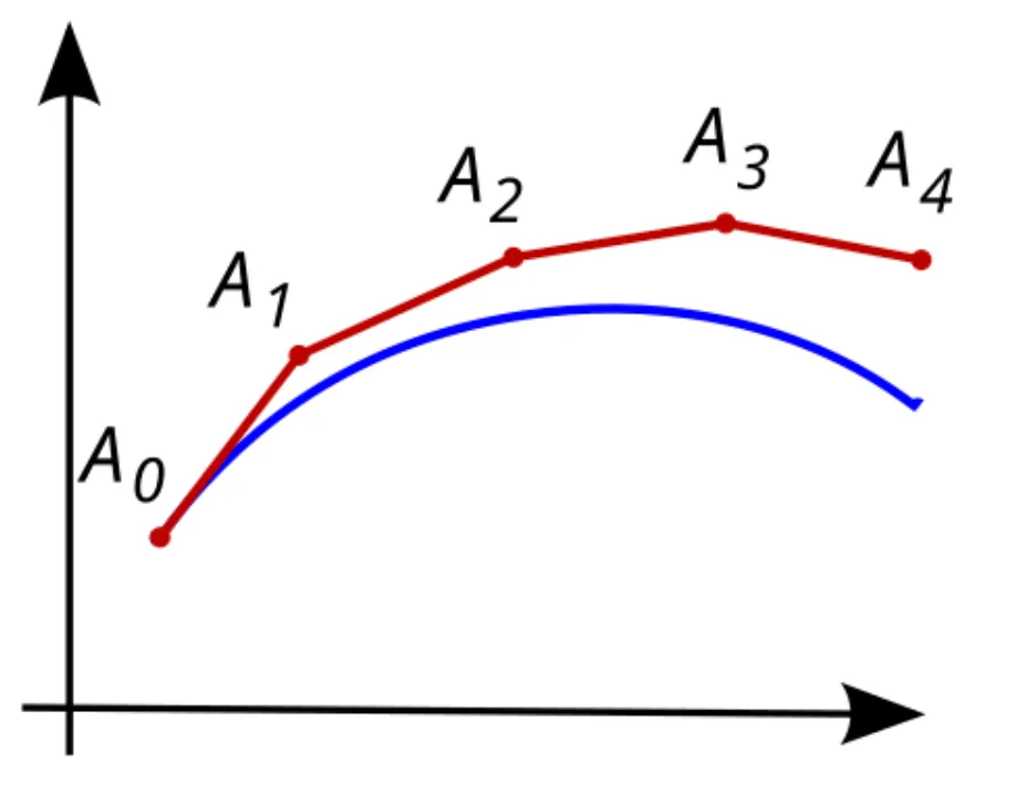
With this update rule, HiPPO can approximate a continuous function that penetrates the cumulated input points .
Below briefly illustrates how is updated as well as the corresponding function .
The authors experimented a reconstruction experiment: while allowing the number of coefficients up to 256, HiPPO took elements from continuous-time band-limited white noise process and succeeded to reconstruct the whole input with relatively small error compared to other RNN baselines.
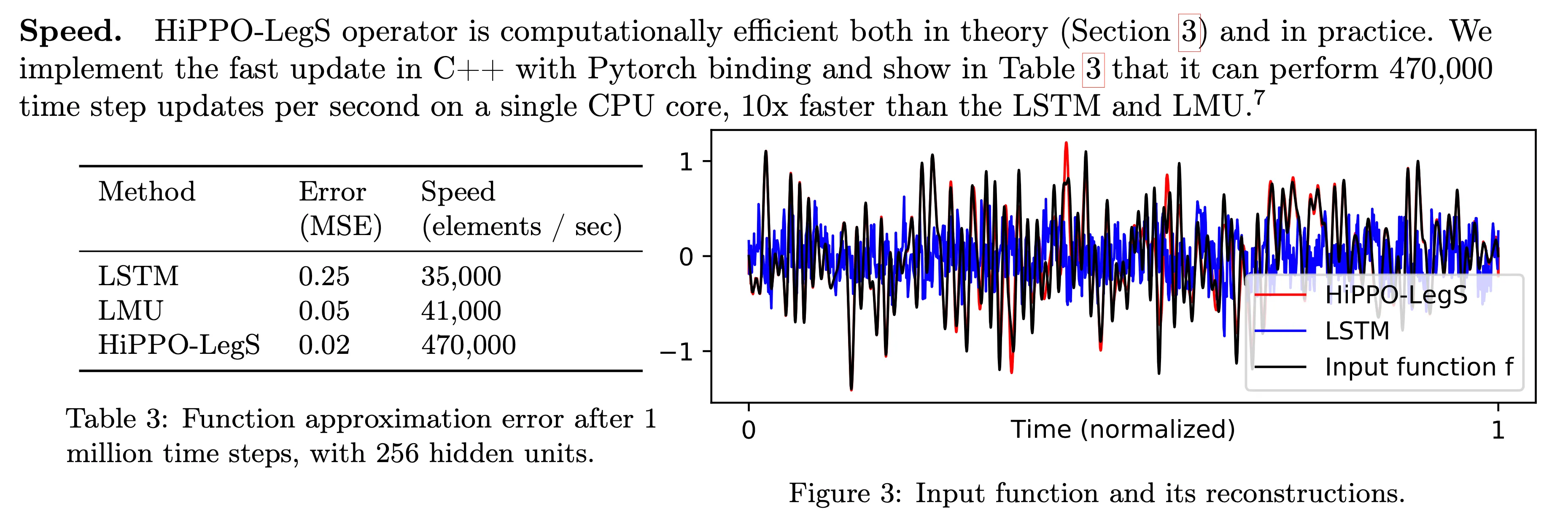
This is quite intriguing, since the parameters and are NOT learnable parameters: they are simply a matrix and a vector filled with constant numbers determined by which orthogonal polynomial you choose. So, we can conclude that this math-based update offers greater advantage over letting a neural network to autonomously learn which update is optimal for remembering every token it has taken.
There are various types of orthogonal polynomials, e.g., Legendre polynomials, Laguerre polynomials, or Chebyshev polynomials, and the authors explicitly derived various s and s that correspond to each of them.
Then how can this be actually used for neural network?
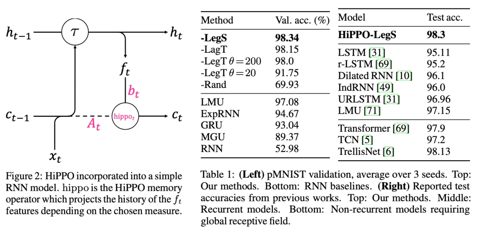
The authors integrated the HiPPO update into RNNs, which typically maintain a hidden state that summarizes the sequence of inputs up to time . In this setup, the hidden state is linearly projected to produce the input for HiPPO, and the corresponding coefficients are updated over time.
Then, instead of feeding just the current input into the RNN’s update function , they used the concatenated input . This modification led to performance improvements on tasks that require learning long-term dependencies, showing that HiPPO summary provided useful additional context for remembering histories.
I spent quite a bit of time explaining HiPPO, but it was because a solid understanding of HiPPO is crucial for grasping the rest of the state-space models that follow.
In the next paper (which I’ll refer to as LSSL for short), the authors take things a step further:
They now generalize and , turning them into learnable parameters.
Combing Recurrent, Convolutional, and Continuous-time Models with Linear State-Space Layers (LSSL)
Albert and his group clearly had a strong desire to extend the strengths of HiPPO into neural network — not just by plugging it into existing architectures, but by building an entirely new kind of network around it.
They propose linear state-space layer (LSSL), one that captures HiPPO’s core ideas as a standalone neural architecture, and something that hadn’t really been explored before.
To begin with, LSSL is suggested as a sequence-to-sequence layer,
which transforms a sequence into a sequence of same length .
Its overview is illustrated well in Figure 1:
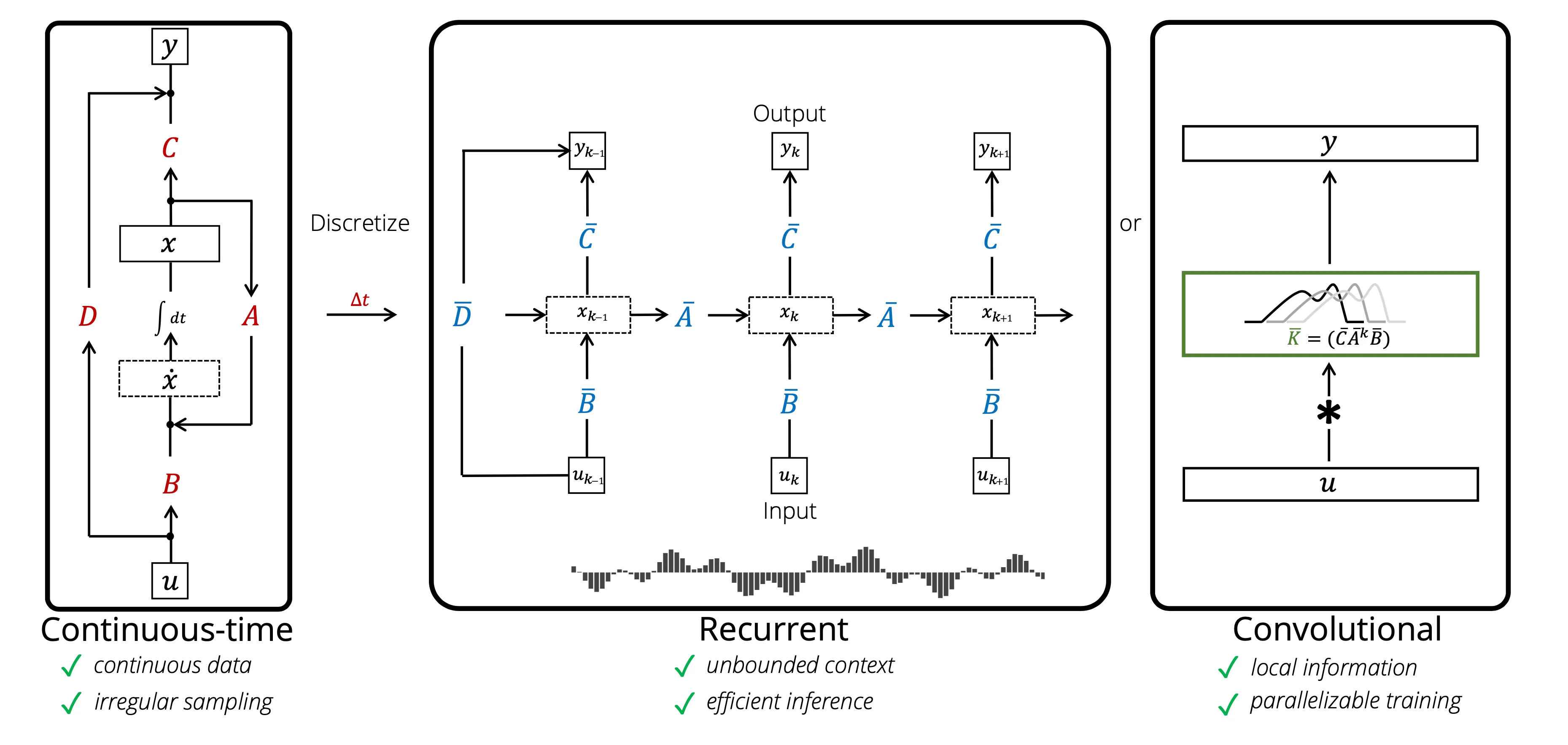
- The input is now replaced with .
- The coefficient is now expressed as .
Their main idea is to keep track of a cumulated summary and use it to generate the output sequence , expecting the output representation to have stronger memory capabilities compared to those produced by typical sequence-to-sequence models.
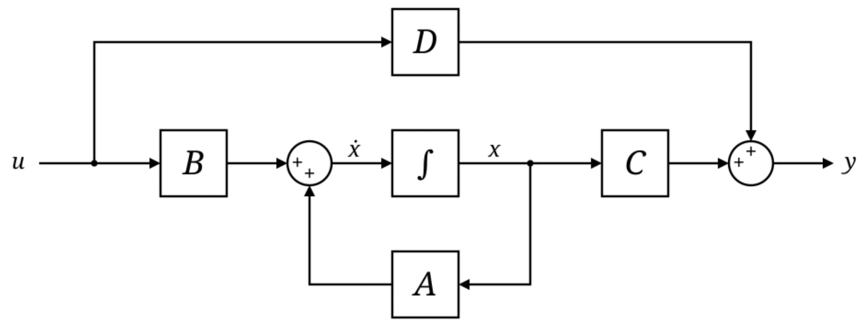
LSSL formulates the sequence-to-sequence layer as follows:
The first row is quite familiar: it’s exactly the same as the HiPPO update, except now and are learnable parameters — we’ll come back to that shortly.
Other parameters and are a linear projection and a scalar weight that interact with and to output , which could be the simplest choice to utilize the summary and the input but interestingly, also a choice that happens to have properties well-studied in the State-space representation from control theory.
But as I read more and more, it turned out that such choice makes many things make sense, especially owing to the well-established theories in control theory.
I’m not really sure if the HiPPO update is inspired by the formulations in control-theory in the first place — but if not, it is quite interesting that two seemingly unrelated theories meet in the middle and one provides theoretical groundings for another. I’ve searched a little, but I haven’t seen any state-space representation from control theory uses the matrix like ones that are derived in HiPPO.
There are three properties that this LSSL formulation provides:
- LSSL is recurrent.
- LSSL is convolutional.
- LSSL is continuous-time.
From the studies we’ve done in HiPPO, we can admit that such a formulation gives recurrent and continuous-time nature — the formulation surely has a recurrent nature, and HiPPO tried to estimate a continuous function that creates the discrete sequence .
But where is this “convolutional” property coming from?
The convolutional layout can be found by unrolling the equation :
If you look at this unrolling process carefully, you might notice that each is obtained by convolving a kernel on a zero-padded sequence .
Since , we can also say (note that ):
Now it becomes clear what the rightmost diagram of Figure 1Show information for the linked content illustrates (although it has omitted the residual connection).
In fact, this concept was not new in control theory, in the name of impulse response :
In signal processing and control theory, the impulse response, or impulse response function (IRF), of a dynamic system is its output when presented with a brief input signal, called an impulse (δ(t)).
…
the impulse response describes the reaction of the system as a function of time.
Roughly speaking, it’s a system’s response to an impulse input (a sudden high-magnitude input).
In a linear state-space system (or an LTI system, a system that follows thisShow information for the linked content), the system output is called impulse response when the input is impulse (Dirac delta ).
This concept allows us to compute the output of a linear state-space system for any arbitrary input by convolving the impulse response with the input. And as you might guess,
the discrete convolution kernel that represents the impulse response is exactly .
The convolutional formulation of LSSL already benefits from ideas rooted in control theory —
but one particularly nice insight borrowed from that field is the following (quoted directly from LSSL paper):
a convolutional filter that is a rational function of degree can be represented by a state-space model of size . Thus, an arbitrary convolutional filter can be approximated by a rational function (e.g., by Padé approximants) and represented by an LSSL.
This strongly supports the expressive power of LSSL: it not only captures a broad range of behaviors that convolution kernels can model, but also sequential modeling capabilities (and gating mechanisms as well, shown by authors with lemmas) of RNNs.
In the meantime, I hope you still keep track of obtaining generalized Show information for the linked content and Show information for the linked content.
As LSSL inherits good points of CNN and RNNs, it also inherits negative sides of CNN and RNNs:
they both poorly handle long-term dependencies.
That’s where the authors come up with using HiPPO’s parameters and .
Since using and derived from orthogonal polynomials already showed benefits in learning long-term dependencies, the authors hypothesized that learning parameterized versions of and , while staying within the space defined by those derivations, might be even more effective.
The idea is this: if we can identify the common structure shared by s and s that are derived from different orthogonal polynomials, we can embed that structure as a constraint. Then, the network is free to learn the rest — adapting the parameters as needed, but always within the “solid shape” imposed by the orthogonal polynomial framework.
So, how do and look like?
At this point, it is worth to note how orthogonal polynomial bases are created, since we need to deal with structures of and derived by arbitrary orthogonal polynomials.
How orthogonal polynomials are formed
Every orthogonal polynomial is tied with their specific weight function , which determines their characteristics. For example, choosing a uniform yields Legendre polynomials, and defined on yields Chebyshev polynomials.
Given a certain , you can repeat Gram-Schmidt process to obtain orthogonal polynomials that satisfy
So, by deriving and from an arbitrary weight function , we can move toward our goal of identifying “the structure”.
This derivation is in fact a very tedious job to do (it’s in Appendix D.2), since it becomes impossible to explicitly write how looks like and you rather need to rely on their properties to carry out the derivation.
I will not explain this process — but the authors ended up concluding two remarks.
- While the vector has no specific structure (highly varies by the measure ),
the matrix is a low recurrence-width (LRW) matrix. - For some weight functions (that are well known to produce good properties — specifically,
: corresponds to Hermite polynomials,
: corresponds to Jacobi Polynomials, and
: corresponds to Laguerre polynomials),
the matrix becomes 3-quasiseparable.
I know — all these unfamiliar math terms can feel overwhelming. But don’t worry, here’s a very quick breakdown:
- An LRW matrix is a special kind of square matrix related to orthogonal polynomials.
LRW matrices is a subset of square matrices that allow near-linear operation to compute matrix-vector multiplication, so it has advantage over other matrices in computational efficiency. - A quasiseparable matrix is a matrix whose off-diagonal blocks have low rank. The number in front (like "1-quasiseparable") specifies constraints on the ranks of those submatrices, which directly impacts how efficiently we can compute with them.
These structural properties not only reveal something fundamental about how is structured, but also bring a major computational advantage. In particular, they enable efficient construction of this kernelShow information for the linked content, which involves computing powers of — typically an expensive operation that becomes much faster thanks to this structure.
It is quite an fascinating breakthrough: we usually trade off efficiency for better performance.
But in this case, the structure of gives us both.
We tested that LSSLs with random matrices (normalized appropriately) perform very poorly (e.g., 62% on pMNIST).
In my opinion, this part is the most beautiful aspect of state-space models:
their ability to model long-term dependencies and maintain computational efficiency — all grounded in elegant mathematical principles.
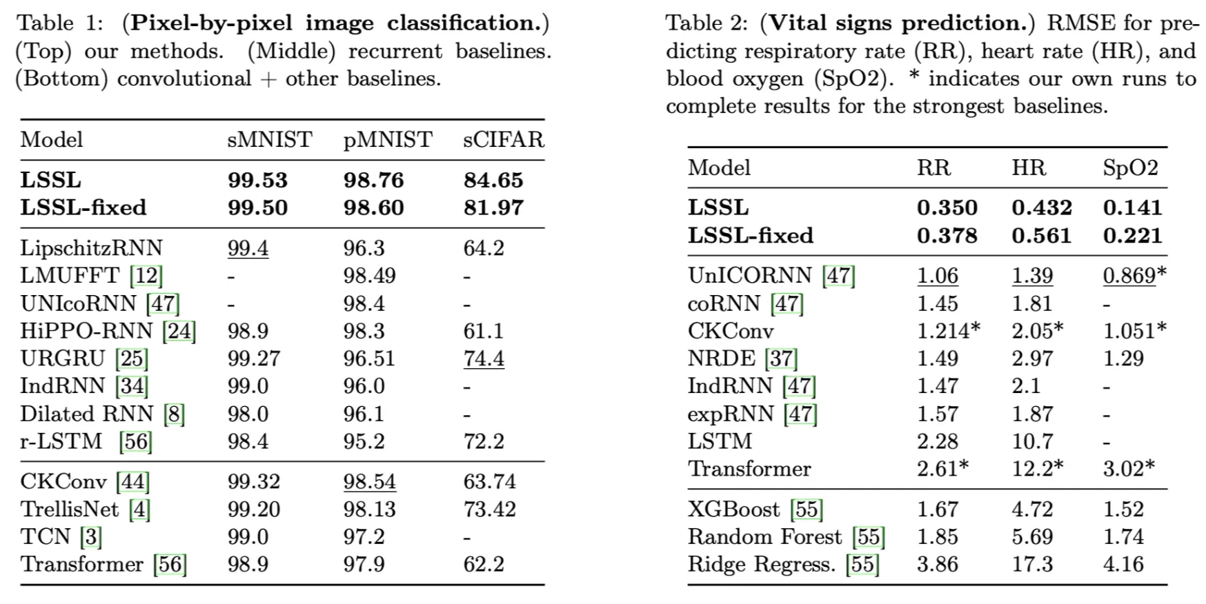
One more impressive point of LSSL is that LSSL-fixed — a network that occupies fixed and from HiPPO — already surpasses other model. Making them learnable can further boost the performance.
Efficiently Modeling Long Sequences with Structured State Space (S4)
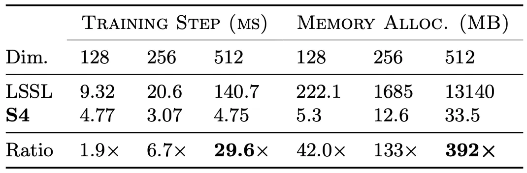
Although LSSL already looks like a fantastic model, they actually had concerns:
(quoted from LSSL)
Sections 1 and 3 and Fig. 1 mention that a potential benefit of having the recurrent representation of LSSLs may endow it with efficient inference. While this is theoretically possible, this work did not experiment on any applications that leverage this. Follow-up work showed that it is indeed possible in practice to speed up some applications at inference time.
…
A follow-up to this paper found that it is not numerically stable and thus not usable on hardware.
In fact, LSSL was NOT really occupying efficiency derived from the structure of due to the numerical instability.
This paper shows that the faster algorithm based on the structure of involves the terms that grow exponentially with — the number of state dimensions.
(quoted from S4)
Lemma B.1. When , the fast LSSL algorithm requires computing terms exponentially large in .
…
the largest coefficient is . When this is .
This creates a frustrating paradox — we know there's an efficient algorithm in theory, but it becomes practically unusable due to physical (numerical) limitations of real-world computers.
The authors come up with a new model, S4, that addresses this challenge.
In this case, I’ll skip most of the model details, since they involve quite a lot of advanced math. But the good news is, you don’t need to understand all the technical details to follow the main idea. The very brief summary of this algorithm is as follows:
- To simplify the problem, the authors restrict the scope of matrix to only few cases considered in HiPPO: ones obtained by using Laguerre and Legendre polynomials.
The authors figured that these matrices share a common structure of
(normal matrix + low rank matrix), in short, NPLR (Normal Plus Low Rank). - The main problem of generating the convolution kernel was to compute the matrix ’s power.
Under the assumption of now being NPLR, authors computed the kernel values by finding an equivalent operation in frequency space.If you want to see a bit more detailed steps, check these out.- Step 1: Move to frequency domain.
Represent the kernel with generating function (a.k.a “z-trasformation” in the literature of control theory).
Intuitively, it is a function that maps from time domain to frequency domain, which can be reverted back to time domain via inverse Fourier transform.
Roughly speaking,
= inverse_fast_fourier_transform(generating_function()). - Step 2: Replace matrix powers with inverses.
The modified representation enables substitution of “power of ” to “inverse of ”. In other words, computing conveniently offers us ’s. - Step 3: Exploit the NPLR structure.
Since is NPLR, we can convert . This can be conjugated into DPLR (Diagonal Plus Low Rank) over , say, . - Step 4: Apply the Woodbury Identity and Cauchy kernel computation algorithm.
This identity reduces the problem of computing the inverse of to the problem of computing the inverse of , which now involves the computation of Cauchy kernel — a well-studied problem that can be solved with near-linear algorithms. - This blog might help for more details.
- Step 1: Move to frequency domain.
With such sophisticated math skills, the authors finally made LSSL an efficient algorithm.
More importantly, it still maintains its strength: learning long-range dependencies.
Mamba: Linear-Time Sequence Modeling with Selective State Spaces
Now here comes Mamba. To briefly summarize the current flow, we can state it like:
- HiPPO established a method to summarize and recover long sequences using orthonormal polynomials, and first invented the notion of the matrix .
- LSSL formulated the state-space models (SSMs), generalized the matrix , and succeeded to transform it into a learnable structure.
- S4 enhanced LSSL by genuinely employing the efficient structure of .
There has been a lot of advance in SSMs between S4 and Mamba.
The notable models are followings:
- DSS (NeurIPS 2022):
Showed that diagonal approximation of the structured matrix can achieve performance comparable to S4’s DPLR formulation. - S4D (NeurIPS 2022):
Suggested simpler, faster, and theoretically more sound diagonal approximation of , with minimal expressivity loss compared to S4’s . - S4ND (NeurIPS 2022):
Proposed the extension of S4 that can handle multi-dimensional data. - S5 (ICLR 2023):
Established the Multi-Input-Multi-Output (MIMO) framework of SSM, and adopted Blelloch parallel scan for faster, parallelizable computation of the kernel .
For 2 years after the advent of S4, the researchers in state-space models have succeeded to simplify the structure of into diagonal matrix, established its initialization, and enabled even faster computation for the kernel () construction.
Mamba’s motivation was something apart from these problems. It rather tackled the foundational problem of SSMs: “content-awareness”.
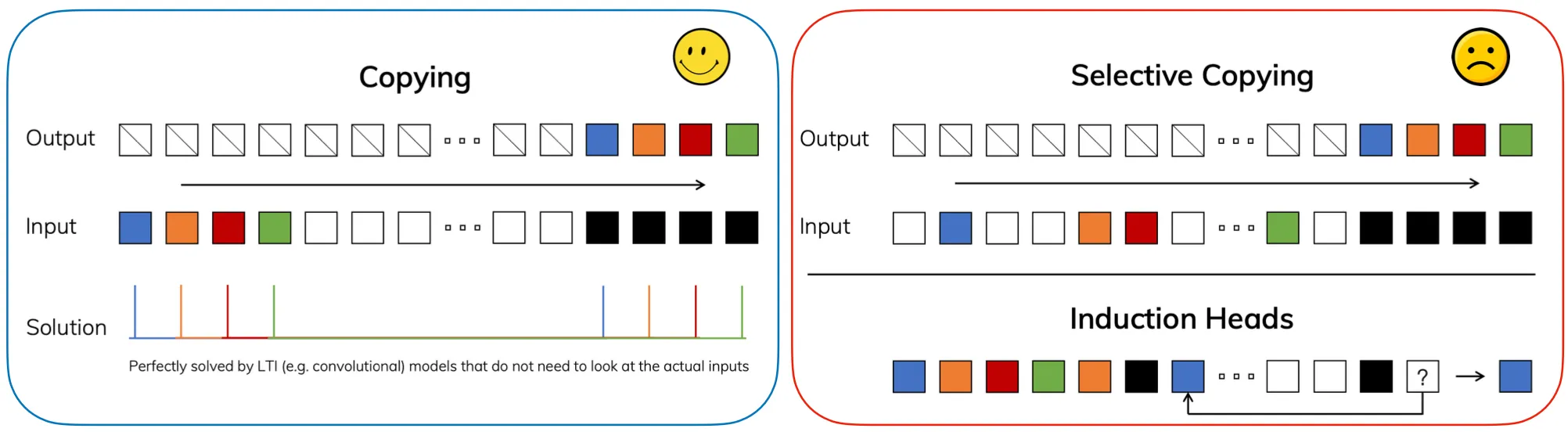
Selective copying task example: move the first colored blocks in the input sequence to the tail.
The authors observed that SSMs are good at the Copying task, which simply requires memorizing and reproducing the entire sequence of input tokens in order. However, they perform much worse on the Selective Copying task, a slightly more challenging variant that requires content-awareness: the model must still preserve the order of tokens, but only for a specific subset (e.g., the “colored” tokens).
This really highlights both the strength and the limitation of SSMs. On the one hand, they’re fantastic at memorization — if you ask them to store a sequence, they’ll remember every element faithfully. On the other hand, that’s also the problem: they remember everything with equal importance. It is quite obvious from its initial derivation — using orthogonal polynomial to reconstruct all of them (although the weight function somehow governs where should SSMs focus more to lower the approximate error, but it still does not change depending on the input). There’s no built-in mechanism to filter out noise or emphasize what really matters.
And that’s exactly where the gap shows up when we think about scaling SSMs toward LLM-like reasoning. Human-like reasoning doesn’t come from replaying every detail word-for-word — it comes from blurring out the unimportant stuff, compressing the input into abstract concepts, and then reasoning from those abstractions. Without that ability, SSMs risk getting stuck as great memorization machines, but not great reasoning machines.
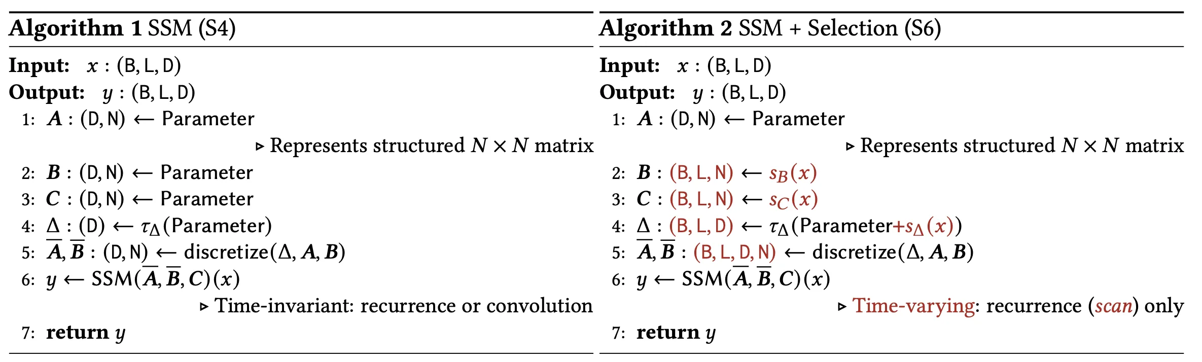
The idea to make SSMs aware of the input contents was quite simple and straightforward: the authors let the model parameters determined by the input itself.
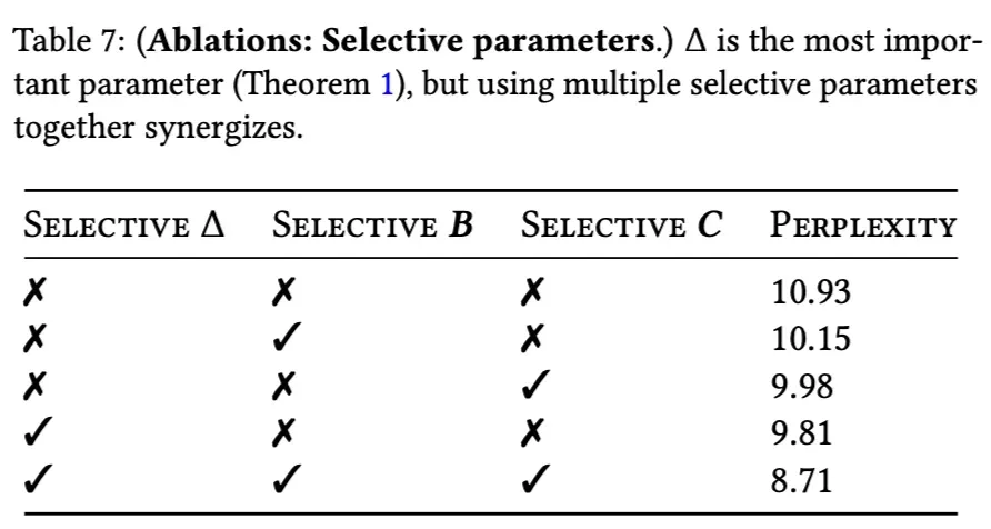
Above is one ablation from the manuscript that shows the performance gain from input-dependency (selectivity). Depending on the context, the input can “choose” a slightly different version of the model to pass through. The effect is quite notable: instead of rigidly applying the same dynamics everywhere, the model adapts its parameters on the fly, shaping itself to better process whatever information is currently in front of it.
At first glance, making parameters input-dependent feels like a pretty straightforward upgrade. In fact, letting a model adapt to its context is not exactly a new idea in machine learning.
But within the world of SSMs, it was actually a big deal.
Why? Remember that SSMs have been through a lot of attempts to handle its speed on top of its elegant theory: LSSL was too slow, S4 came up with sophisticated fast-working algorithms, and subsequent works devised diagonal to compute the kernel even faster. On top of this flow, adopting input-dependent parameters will add a heavy computational burden, which couldn’t be justifiable unless the authors invent another breakthrough to enhance its efficiency.
This time, the authors took engineering-type of approach: hardware-aware algorithm.
I am not an expert in this field, so I will list my understandings about this algorithm in easy, understandable words.
- Apparently there are two parts in GPU that are mainly responsible for feed-forward process.
- High-bandwidth memory (HBM)
- Static Random-Access Memory (SRAM)
- HBM allows greater memory but it’s slower in computation, while SRAM is the opposite.
- The biggest efficiency bottleneck comes from memory I/O in GPU. Modern GPUs tend to compute the intermediate state ( of this equationShow information for the linked content) in HBM. If one could move this computation in SRAM (but this time without saving the intermediate states) it bypasses such memory read/write operations. Plus, it has better computation speed.
- For backpropagation one needs to re-compute the intermediate states since they are not stored during feed-forward. (just like gradient checkpointing)
- For sequence length 𝐿 too long where the sequence cannot fit into SRAM (which is much smaller than HBM), the sequences split into chunks and perform the fused scan on each chunk.
In short, they moved slower, tricky process of SSM computations to fast SRAM while handling the insufficient memory of SRAM.
This almost feels like a cheat code; if we were aware of such mechanisms and had abilities to implement these, applying this type of algorithms could eventually enhance most of the networks we want to design. In fact, this is done with sophisticated CUDA-level programming with the aid of Albert’s former labmate, Tri Dao, who is known for efficient hardware-aware algorithms and also the author of renowned FlashAttention.
Albert and Tri had already worked on fast computation using structured matrices, so it isn’t surprising that they work on efficient algorithm to construct with structured matrix . Combining these matrix structures with hardware-aware design might well have been their ultimate recipe for improving the algorithm.
Anyways, it is actually not as simple as it sounds. You’ll need some serious level of CUDA-level coding skills and high-level understanding of GPU… or a smart labmate willing to handle that part for you.
On top of this algorithm, Mamba additionally introduced interesting insights related to Mamba block design or initialization of , but I won’t describe all of them in this post.
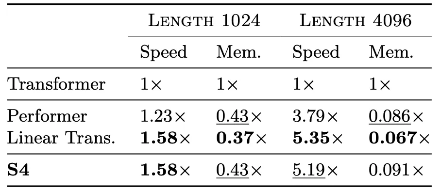
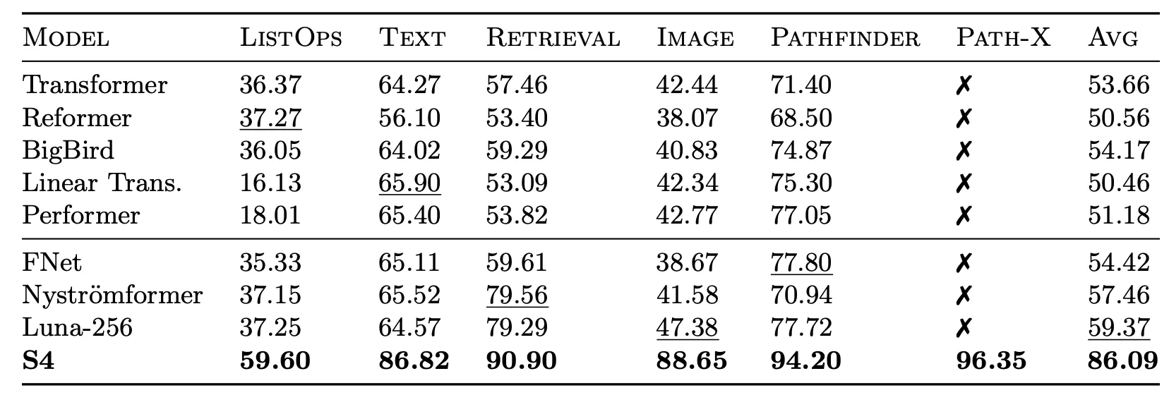
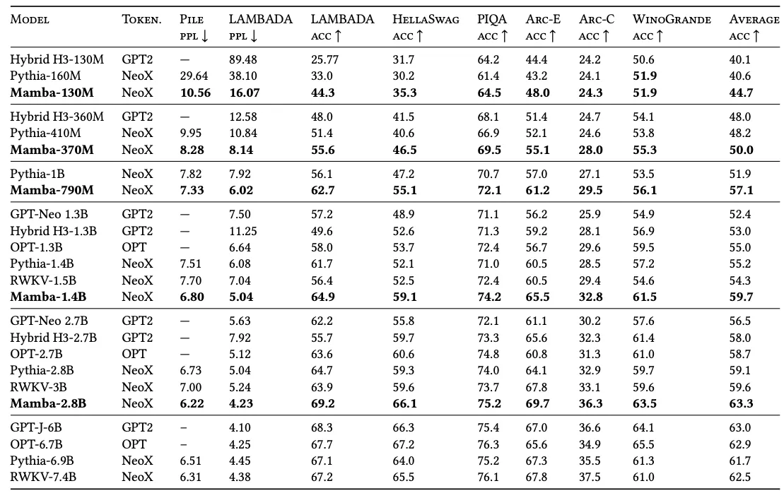
From the broader view of SSM evolution, Mamba marks a real milestone — it’s the first time SSMs stood toe-to-toe with Transformers, matching their performance on tough benchmarks while using less computation.
Mamba is the first attention-free model to match the performance of a very strong Transformer recipe (Transformer++) that has now become standard, particularly as the sequence length grows.
Closing thoughts

Tracing the evolution of SSMs has been fascinating to me because it really shows how theory, computation, and creativity keep bouncing off each other.
LSSL started as this mathematically elegant idea but hit the wall of numerical infeasibility. S4 then came in like a clever hack, finding mathematically equivalent operation that works in practice. From there, diagonal approximations (DSS, S4D), multidimensional extensions (S4ND), and efficient kernels (S5) kept pushing the boundaries. Along the way, we saw SSMs shine at memorizing long-term context, but also bump into the limits of content-awareness — a reminder that remembering everything isn’t the same as understanding.
And now, with Mamba, it feels like SSMs have finally stepped into the big league. They now stand next to Transformers, but with a greater efficiency and better long-term context understanding.
I hope this journey made Mamba’s seemingly unrelatable connection between its structure and its performance much clearer, and maybe even sparked a few ideas for your own research too!